凸优化与非凸优化
凸优化:凸优化在某种意义上说较一般情形的数学最优化问题要简单,譬如在凸优化中局部最优值必定是全局最优值。

非凸优化:

对于凸优化来说,局部最小就是全局最小,因此问题变得简单。
平滑与非平滑
平滑:

处处可导
非平滑:

第二章 无约束优化(线搜索框架下)
1. 梯度法(最速下降法)
梯度(gradient):增长最快的方向,导数的高维扩展
先回答需要考虑的问题:
- 负梯度方向,“速”非快
- 一维搜索求$\lambda_k$,使得
- 最速下降法适用于寻优过程的前期迭代或作为间插步骤,当接近极值点时,宜选用收敛快的算法.
3. 共轭梯度法


正如从上面例子中看到的,简单梯度下降算法的一个问题是,它试着摇摆穿越峡谷,每次跟随梯度的方法,以便穿越峡谷。共轭梯度通过添加摩擦力项来解决这个问题: 每一步依赖于前两个值的梯度然后急转弯减少了。
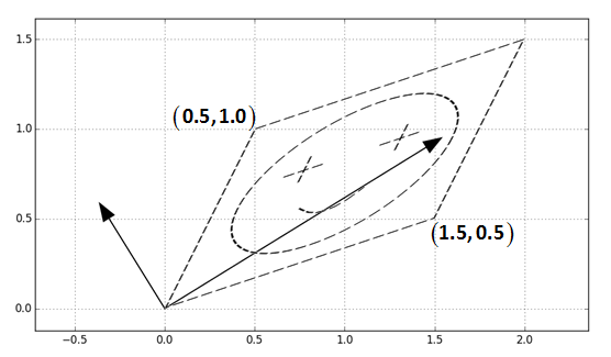
首先理解特征值:
- 线性变换$\mathcal L$
- $n \times 1$向量$u$ $\Longrightarrow$ 特征向量
比例引子$\lambda$ $\Longrightarrow$ 特征值
也就是经过一个线性变换后,在沿着$u$的方向上只发生了缩放,原来的方向不变,就好像这个方向是枚“定海神针”,牢牢定义了这个线性变换。

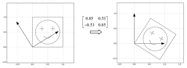
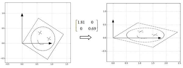

- 第一步:旋转 $U^T$
- 第二步:$\Sigma$对角矩阵,相当于进行缩放
- 第三步:旋转 $U$,转回去
什么是共轭
- $G$: $n \times n$对称正定矩阵
- ${p_0,p_1,\ldots,p_k}$: 非零向量组合
若满足
说明这一组向量有$A$-正交性/共轭性,或者说是线性无关(n维至多n个),从这儿也能看出来,共轭是正交的扩展:当$A$为单位向量$I$时即是正交,就好像梯度是导数的扩展(?)
- 所谓共轭方向方法即是所有使用共轭向量作为梯度更新方向的算法。
- 共轭梯度算法则是在迭代过程中利用梯度下降法来更新共轭向量组。
从任意点$x_0$出发,沿任意下降方向$p_i$做直线搜索得到$x_1$,接着沿与$p_i$共轭的$p_j$方向搜索,反复迭代
2. Newton Method
牛顿法使用局部二元近似来计算跳跃的方向。为了这个目的,他们依赖于函数的前两个导数梯度和Hessian。
- On a real quadritic surface it jumps to the minimum in one step.
- Unfortunately, with only a million weights, the curvature matrix has a trillion terms and it is totally infeasible to invert it.
Curvature Matrices: H(w)
- Each element in the curvature matrix specifies how the gradient in one direction changes as we move in some other direction.
- The off-diagonal terms correspond to twists in the error surface.
- The reason steepest descent goes wrong is that the gradient for one weight gets messed up by the simultaneous changes to all the other weights.
- The curvature matrix determines the sizes of these interactions.
The genuinely quadratic durface is the quadratic approximation to the true surface.
$g(x)$是quadratic$f(x)$的导数,求$f(x)$的极小点则是求$g(x)$的零点,于是有:
一维
割线法(secant)
推广至高维
Hessian矩阵$\mathbf H=\nabla^2 f(\mathbf x)$
Lipschitz连续
优点
- 二阶收敛
也可能不收敛
缺点
- 要求Hessian矩阵要可逆
- 需要计算二阶导数和逆矩阵,计算量和存储量 开销较大
2. Quasi-Newton Method
In the Hessian-free method, we make an approximation to the curvature matrix and then, assuming that approcimation is correct, we minimize the error using an efficient technique called conjugate gradient. Then we make another approximation to the curvature matrix and minimize again.
- For RNNs its important to add a penalty for changing any of the hidden activities too much.
近似Hessian的逆矩阵
无记忆拟牛顿法和共轭梯度法联系最紧密
BFGS
(Broyden-Fletcher-Goldfarb-Shanno算法) 改进了每一步对Hessian的近似。
L-BFGS:
限制内存的BFGS介于BFGS和共轭梯度之间: 在非常高的维度 (\gt 250) 计算和翻转的Hessian矩阵的成本非常高。L-BFGS保留了低秩的版本。此外,scipy版本, scipy.optimize.fmin_l_bfgs_b(), 包含箱边界:
Conjugate Gradients(CG)
- Use a sequence of steps each of which finds the minimum along one direction.
Make sure that each direction is "conjugate" to the previous directions so you do not mess up the minimization you already did.
conjugate: when you go in the new direction, you do not change the gradients in the previous direction.
After
Nstep, conjugate gradient is guaranteed to find the minimum of N-dimensional quadratic surface.Conjugate gradient can be apllied to a non-quadratic error surface and it usually works quite well.
- The HF optimizer uses CG for minimization on a genuinely quadratic surface where it excels.
3.线性搜索
- 搜索方向$d_k$
步长因子$\alpha_k$
目标就转化成了$\phi(\alpha_k) \lt \phi(0)$。
精确线性搜索
目标在于沿着$d_k$方向让目标函数达到极小。这样得到的$\alpha_k$叫精确步长因子。
- $A$ : 半正定对称矩阵
精确步长(stride)就可以表示出来了:
正交条件
不精确线性搜索
进退法——确定初始搜索区间
高-低-高
二次收敛性
当目标函数是二次函数时,共轭方向法最多经过$N$步迭代($N$=向量维数),就可达到极小值点。
bb法
第三章 有约束优化
- $\mathbf c(x)=(c_1(x),\ldots,c_n(x))^\top$
- $\mathbf \lambda=(\lambda_1,\ldots,\lambda_n)^\top$
- $\nabla_xL(x,\mathbf \lambda)=\nabla f(x)-\mathbf \lambda^\top \nabla \mathbf c(x)=0$
- $\nabla_\lambda L(x,\mathbf \lambda)=-\mathbf c(x)=0$

$-1 \lt x_1 \lt 1$
$-1 \lt x_2 \lt 1$
1. 信赖域
- 当前点,用二次函数近似当前函数:$q_k(\cdot)\approx f(x)$
- 求解$q_k$极小值点作为下一次试探点
先确定区域$\Delta k$,可选不同范数
- 无穷范数:$\max{|x_i|}$
$s_k^c=-\tau_k \frac{\Delta k}{||g_k||}g_k$
$\tau_k=\begin{cases} 1, &g_k^\top B_kg_k\leq 0\cr \min{\frac{||g_k||^3}{\Delta kg_k^\top B_kg_k},1}, &otherwise \end{cases}$
动态调整
折线法
$\Delta_k=\frac 12$,第$k$步求解子问题时用双折线法求解
由于$\mathbf x_k=(1,1)^\top$,则
$g_k=\nabla f(\mathbf x_k)=\left[
\begin{matrix}
4x_1^3+2x_1\2x_2
\end{matrix}
\right]$
,从而得到$g_k=(6,2)^\top$。
同理可得:
由于$||s_k^c||\cong 0.496 \Delta_k$,从而需要计算牛顿步$s_k^{\hat N}$,有
由于$||s_k^{\hat N}||\gt\Delta_k$,故取双折线步长为$s_k=s_k^c+\lambda(s_k^{\hat N}-s_k^c),\lambda \in (0,1)$,使得$|s_k^{\hat N}||=\Delta_k$。
解二次方程:
得$\lambda \cong 0.876$。因此,
2. 积极集法
* $y\in {y|\nabla_ic(x^*)^\top y=0,\forall i}$在$c(x)=0$这个超平面上,等价于在无约束情况$y\in \mathbb R^n$。
* 用脚标的集合表示哪些到达边界约束。

  * $x^_$处的积极集:$I(x^_)={i\|c_i(x^)=0}\Longleftrightarrow \exists \lambda_0,\ldots,\lambda_n\geq0  s.t. \lambda_0\nabla f(x^)-\sum_{i=1}^m \lambda_i^_ \nabla_ic_i(x^_)=0$
  * 如果$\nabla c_i(x^)(i\in f(x^))$线性无关,则存在向量$\mathbf \lambda^$,使得$\nabla f(x^)-\sum_{i=1}^m \lambda_i^_ \nabla_ic_i(x^_)=0,\lambda_i^_\geq0$对偶变量,$\lambda_i^_c_i(x^*)=0$互补松弛条件$

  * 带约束问题$\rightarrow$方程组求解
* 目标函数下降方向集合$F={d\|\nabla f(x)^\top d\lt0}$
* 可行方向:$D={d|\nabla c_i(x)^\top d\geq0,i\in I(x)}$
Gordan定理:$\mathbf A\mathbf x \gt 0$有解$\Longleftrightarrow$不存在$\mathbf y \geq 0$使得$\mathbf A^\top \mathbf y=0$
举例:用积极集法求解
变为标准型:
记上面的约束为1到3
计算$\nabla f(\mathbf x)=(2x_1-x_2-1,4x_2-x_1-10)^\top$。因为$\mathbf x^1=(\frac 27,\frac {18}7)^\top$,所以有效约束$I(\mathbf x^1)={1}$,$\nabla f(\mathbf x^1)=(-3,0)^\top$,相应的等式约束问题为
由等式约束问题的一阶必要条件得到
求解方程组得到$d_1=\frac 12, d_2=\frac 94,\lambda_1=\frac 34$,


即$\mathbf \lambda=(\frac 34,0,0)^\top$,$\mathbf x^2=(\frac 12,\frac 94)^\top$是最优解。
3. 直接法
1. $x_1\in \mathbb R^n,d_1,\ldots,d_n线性无关$
2. $x_1$沿$d_1$线性搜索得$x_2$,即$x_2$是$f(x)$在${z\|z=x_1+\alpha_1 d_1}$上的极小值点
3. $\beta_1,\ldots,\beta_n,\nu^{(1)}=x_2+\beta_2d_2$,令$d_2=\nu^{(2)}-x_2$,$\nu^{(2)}$是$f(x)$在${z\|z=\nu^{(1)}+\alpha_1 d_1}$上的极小值点
   * $\nabla f(\nu^{(1)})^\top d_1=0,\nabla f(x_2)^\top d_1=0$
   * $d_2^\top Hd_1=0$(共轭,$d_2=\nu^{(2)}-x_2$)
4. 令$d_3=\nu^{(3)}-x_3$,则$\nu^{(3)}$是$f(x)$在${z\|z=x_1+\alpha_1 d_1+\alpha_2 d_2}$上的极小值点
5. $x_{k+1}$是$f(x)$在${z\|z=x_1+\sum_{i=1}^k\alpha_i d_i}$上的极小值点,令$d_{k+1}=\nu^{(k+1)}-x_{k+1}$
Reference
- 《最优化理论与方法》陈宝林
- 《非线性优化计算方法》袁亚湘
- 《Numerical Optimization》Jorge Nocedal
术语表
二阶(quadratic)
其他
0.618法
用0.618法寻找最佳点时,虽然不能保证在有限次内准确找出最佳点,但随着试验次数的增加,最佳点被限定在越来越小的范围内,即存优范围会越来越小。用存优范围与原始范围的比值来衡量一种试验方法的效率,这个比值叫精度。用0.618法确定试点时,每一次实验都把存优范围缩小为原来的0.618.因此,n次试验后的精度为:
KKT条件

In mathematical optimization, the Karush–Kuhn–Tucker (KKT) conditions (also known as the Kuhn–Tucker conditions) are first order necessary conditions for a solution in nonlinear programming to be optimal, provided that some regularity conditions are satisfied. Allowing inequality constraints, the KKT approach to nonlinear programming generalizes the method of Lagrange multipliers, which allows only equality constraints. The system of equations corresponding to the KKT conditions is usually not solved directly, except in the few special cases where a closed-form solution can be derived analytically. In general, many optimization algorithms can be interpreted as methods for numerically solving the KKT system of equations.
编程
footnote1. 《2.7 数学优化:找到函数的最优解》 ↩