神经网络结构
Multi-Layer Neural Network}
A.3-layer network: Input Layer,Hidden Lyer,Output layer Except input units,each unit has a bias.
preassumption calculation}
Hidden Layer: Specifically, a signal $xi$ at the input of synapse $i$ connected to nueron $j$ us multiplied by the synaptic weight $w{ji}$ $i$ refers input layer,$j$ refers hidden layer.$w{j0}$ is the bias.$x{0}=+1$
- Each neuron is represented by a set of linear synaptic links, an externally applied bias, and a possibly nonlinear activation link.The bias is represented by a synaptic link connected to an input fixed at $+1$.
- The synaptic links of a neuron weight their respective input signals.
- The weighted sum of the input signals defines the induced local field of the neuron in question.
- The activation link squashes the induced local field of the neuron to produce an output.
Output layer: $f()$ is the activation function.It defines the output of a neuron in terms of the induced local field $net$ .
{% math %}
\xymatrix {
 %x_{0}=+1 \ar[ddr]|(0.6){w_{j0}} &  &\\
 %x_{1} \ar[r]|(0.6){w_{j1}} & B & C\\
 %x_{2} \ar[r]^(0.6){w_{j2}} & net_{j} \ar[r]^(0.6){f()} & y_{j} \\
 x
}
{% endmath %}
For example:
$n_{H}$is the number of hidden layers.
So:
The activate function of output layer can be different from hidden layer while each unit can have different activate function.
BP Algorithm
The popularity of on-line learning for the supervised training of multilayer perceptrons has been further enhanced by the development of the back-propagation algorithm. Backpropagation, an abbreviation for "backward propagation of errors",is the easiest way of supervised training.We need to generate output activations of each hidden layer. The partial derivative $\partial J /\partial w_{ji}$ represents a sensitivity factor, determining the direction of search in weight space for the synaptic weight Learning:
the instantaneous error energy of neuron $j$ is defined by
In the batch method of supervised learning, adjustments to the synaptic weights of the multilayer perceptron are performed \emph{after} the presentation of all the $N$ examples in the training sample $\mathcal T$ that constitute one \emph{epoch} of training. In other words, the cost function for batch learning is defined by the average error energy $J(w)$.
- firstly define the training bias of output layer:
input->hidden
仿射层(Affine Layer)
神经网络中的一个全连接层。仿射(Affine)的意思是前面一层中的每一个神经元都连接到当前层中的每一个神经元。在许多方面,这是神经网络的「标准」层。仿射层通常被加在卷积神经网络或循环神经网络做出最终预测前的输出的顶层。仿射层的一般形式为 y = f(Wx + b),其中 x 是层输入,w 是参数,b 是一个偏差矢量,f 是一个非线性激活函数。
多层感知器(MLP:Multilayer Perceptron)
多层感知器是一种带有多个全连接层的前馈神经网络,这些全连接层使用非线性激活函数(activation function)处理非线性可分的数据。MLP 是多层神经网络或有两层以上的深度神经网络的最基本形式。
反向传播(Backpropagation)
反向传播是一种在神经网络中用来有效地计算梯度的算法,或更一般而言,是一种前馈计算图(feedforward computational graph)。其可以归结成从网络输出开始应用分化的链式法则,然后向后传播梯度。反向传播的第一个应用可以追溯到 1960 年代的 Vapnik 等人,但论文 Learning representations by back-propagating errors常常被作为引用源。
技术博客:计算图上的微积分学:反向传播(http://colah.github.io/posts/2015-08-Backprop/)
通过时间的反向传播(BPTT:Backpropagation Through Time)
通过时间的反向传播是应用于循环神经网络(RNN)的反向传播算法。BPTT 可被看作是应用于 RNN 的标准反向传播算法,其中的每一个时间步骤(time step)都代表一个计算层,而且它的参数是跨计算层共享的。因为 RNN 在所有的时间步骤中都共享了同样的参数,一个时间步骤的错误必然能「通过时间」反向到之前所有的时间步骤,该算法也因而得名。当处理长序列(数百个输入)时,为降低计算成本常常使用一种删节版的 BPTT。删节的 BPTT 会在固定数量的步骤之后停止反向传播错误。
论文:Backpropagation Through Time: What It Does and How to Do It
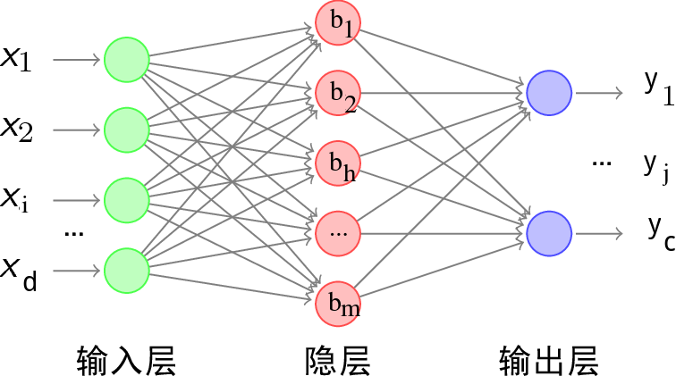
给定训练集$D={(x_1,y_1), (x_2,y_2),\ldots,(x_m,y_m)}$,$x_i \in \mathbb R^d$,$y_i \in \mathbb R^c$,即输入实例由d个属性描述,输出$c$维实值向量.
下图给出了一个拥有$d$个输入神经元、$m$个隐层神经元、$c$个输出神经元的多层前馈网络结构:
- 隐层第$h$个神经元的阈值用$\gamma _h$表示,
- 输出层第$j$个神经元的阈值用$\theta_j$表示。
- 输入层第$i$个神经元与隐层第$h$个神经元之间的连接权为$v_{ih}$;
- 隐层第$h$个神经元与输出层第$j$个神经元之间的连接权为$w_{hj}$;
- 记隐层第$h$个神经元接收到的输入为$\alphah=\sum{i=1}^dv_{ih}x_i$;
- 输出层第$j$个神经元接收到的输入为$\betaj=\sum{h=1}^mw_{hj}b_h$, 其中$b_h$为隐层第$h$个神经元的输出;
- 假设隐层和输出层神经元都使用Logistic函数:
以串行为例,对训练样本$(xk,y_k)$,假定神经网络的输出为$\hat y_k=(\hat y_1^k,\hat y_2^k,\ldots,\hat y_c^k)$,即 则网络在$(x_k,y_k)$上的均方误差(LMS算法)为 根据广义的感知机学习规则对参数进行更新,任意参数$v$的更新估计式为 BP算法基于梯度下降策略,对误差$E_k$,给定学习率$\eta$,有 考虑到$w{hj}$先影响到第$j$个输出层神经元的输入值$\betaj$,再影响到其输出值$\hat y_j^k$,最后影响到$E_k$,有 根据$\beta_j$的定义,显然有 而Logistic函数有一个性质: 于是有 于是得到了BP算法中关于$w{hj}$的更新公式
根据前面的推导 $bh$为第$h$个隐层神经元的输出,即 考虑到$v{ih}$先影响到第$h$个隐层神经元的输入值$\alpha_h$,再影响到其输出值$b_h$,最后影响到$E_k$,有 类似(2)中的$g_j$,有 所以 另外,类似$\Delta \theta _j$
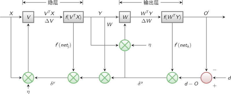
信号流图: