keras
Keras是一个极度简化、高度模块化的神经网络第三方库。基于Python+Theano开发,充分发挥了GPU和CPU操作。其开发目的是为了更快的做神经网络实验。适合前期的网络原型设计、支持卷积网络和反复性网络以及两者的结果、支持人工设计的其他网络、在GPU和CPU上运行能够无缝连接。
基本概念
张量(tensor)
其维数从0到n,axis则对应“轴”的概念。
import numpy as np

a = np.array([[1,2],[3,4]])
sum0 = np.sum(a, axis=0)
sum1 = np.sum(a, axis=1)

print sum0
print sum1
Model模型方法
- evaluate_generator:使用一个生成器作为数据源,来评估模型,生成器应返回与test_on_batch的输入数据相同类型的数据。
数据增强
- featurewise_center的官方解释:"Set input mean to 0 over the dataset, feature-wise."
1. Core 常用层
Permute层
当需要将RNN和CNN链接时可能用到它。用来将输入的维度重排。
keras.layers.core.Permute(dims)
其中dims指定重排的模式(不包括样本数的维度),默认下标从1开始。
Lambda层
keras.layers.core.Lambda(function, output_shape=None, arguments={})
output_shape:函数应该返回的值的shape,可以是一个tuple,也可以是一个根据输入shape计算输出shape的函数
model.add(layers.Lambda(squeeze_dim, output_shape=squeeze_dim_shape))
2. 卷积层
Convolution2D
keras.layers.convolutional.Convolution2D(nb_filter, nb_row, nb_col, init='glorot_uniform', activation='linear', weights=None, border_mode='valid', subsample=(1, 1), dim_ordering='th', W_regularizer=None, b_regularizer=None, activity_regularizer=None, W_constraint=None, b_constraint=None, bias=True)
举例子:
model.add(Convolution2D(64, 3, 3, border_mode='same', input_shape=(3, 256, 256)))
这里的前三个参数是64个3X3的filter的意思,
input_shape = (3,128,128)代表128*128的彩色RGB图像.input_shape不包含样本数的维度,在其内部实现中,实际上是(None,3,128,128)或者(None,128,128,3)
- ‘th’模式下,输入形如(samples,channels,rows,cols)的4D张量
- ‘tf’模式下,输入形如(samples,rows,cols,channels)的4D张量
所以现在model.output_shape == (None, 64, 256, 256)
- subsample:长为2的tuple,输出对输入的下采样因子,更普遍的称呼是“strides”
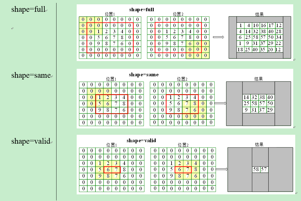
- border_mode=‘full’,same,valid
池化层
MaxPooling2D
keras.layers.pooling.MaxPooling2D(pool_size=(2, 2), strides=None, border_mode='valid', dim_ordering='default')
规范层
BatchNormalization
keras.layers.normalization.BatchNormalization(epsilon=1e-06, mode=0, axis=-1, momentum=0.9, weights=None, beta_init='zero', gamma_init='one')
上一层是激活函数,这一层对它的输出值进行规范化(均值接近0,标准差接近1)
- mode - 0 按样本规范化,默认输入为2D
- axis 指定规范化的轴 (samples,channels,rows,cols)
- 1 沿通道轴(channel) 规范化(4D图像张量)意味着对每个特征图进行规范化
- axis 指定规范化的轴 (samples,channels,rows,cols)
自定义层
ANN
class Network():
    def init(self,sizes):
        self.num_layers=len(sizes)
        self.sizes=sizes
        self.biases=[np.random.randn(y,1) for y in sizes[1:]] #
        self.weights=[np.random.randn(y,x) for x,y in zip(sizes[:-1],sizes[1:])]
- sizes=[2,3,1]
- 权值和偏置是需要初始化,梯度下降算法是在某个点在梯度方向上开始不断迭代计算最优的w和b,所以w,b必须有一个初始值作为起始迭代点。 随机地初始化它们,我们调用了numpy中的函数生成符合高斯分布的数据。
        # Either we have a random seed or the WTS for each layer from a
        # previously trained NeuralNet
        if allwts is None:
            self.rand_gen = np.random.RandomState(training_params['SEED'])
        else:
            self.rand_gen = None
其次这里的w,b表示成向量形式,原因是矢量化编程可以在线性代数库中加快速度,那么到底该怎么表示w,和b呢?让我们从最简单的问题开始,看看最简单的单个神经元:
激活函数
def feedforward(self,a):
for b,w in zip(self.biases,self.weights):
a=sigmoid_vec(np.dot(w,a)+b)
return a
def sigmoid(z):
return 1.0 / (1.0 + np.exp(-z))
sigmoid_vec=np.vectorize(sigmoid)
SGD
def SGD(self,training_data,epochs,mini_batch_size,eta,test_data=None):
随机梯度下降的思想不是迭代所有的训练样本,而是挑一部分出来来代表所有的训练样本,这样可以加快训练速度。换句话说就是,原始梯度下降算法是一个一个地训练,而SGD是一批一批地训练,而这个批的大小就是mini_batch_size,并且这个批是随机挑出来的,而等这些批都训练完了我们叫一次迭代,并且给了它一个更好听的名字叫epochs,eta是学习率$\eta$,test_data是测试数据。看代码!
if test_data:
    n_test=len(test_data)
    n=len(training_data)
for j in xrange(epochs):#开始迭代
    random.shuffle(training_data)#为了是随机地挑选出来的批次,先调用这个函数扰乱训练样本,这样就可以制造随机了
    mini_batches=[training_data[k:k+mini_batch_size]
    for k in xrange(0,n,mini_batch_size)] #索引分批的数据
        for mini_batch in mini_batches:
            self.update_mini_batch(mini_batch,eta) #根据规则更新权值w和偏置b
    if test_data:#在每次迭代结束时,我们都会利用测试数据来测试一下当前参数的准确率
        print "Epoch {0}:{1} / {2}".format(j,self.evaluate(test_data),n_test)
    else:
        print "Epoch {0} complete".format(j)
这里又用到了update_mini_batch方法,它直接把更新w和b的过程单独抽象了出来,这个函数是梯度下降的代码,而只有加上这个函数前面的代码才能叫随机梯度下降。过会我们再来分析这个函数,在迭代完一次(一个epoch)之后,我们使用了测试数据来检验我们的神经网络(已经根据mini-batch学习到了权值和偏置)的识别数字准确率。这里调用了一个函数叫evaluate,它定义为:
def evaluate(self,test_data):
    test_results=[(np.argmax(self.feedforward(x)),y) for (x,y) in test_data]
    return sum(int(x==y) for (x,y) in test_results)
这个函数的主要作用就是返回识别正确的样本个数。其中np.argmax(a)是返回a中最大值的下标,这里我们可以看到self.feedforward(x),其中x是test_data中的输入图像,然后神经网络计算出最终的结果是分类数字的标签,它是一个shape=(1,10)矩阵,比如数字5表示为[0,0,0,0,0,1,0,0,0,0],这时1最大,就返回下标5,其实也就表示了数字5。然后将这个结果和test_data中的y作比较,如果相等就表示识别正确,sum就是用来计数的。
梯度下降算法
$\Delta \nabla_b,\Delta \nabla_w, \nabla_b,\nabla_w$
下面来看看梯度下降的代码update_mini_batch:
def update_mini_batch(self,mini_batch,eta):
    nabla_b=[np.zeros(b.shape) for b in self.biases] #迭代的初值当然是0了,记住这和偏置b的初始值不一样额
    nabla_w=[np.zeros(w.shape) for w in self.weights]

for x,y in mini_batch:#扫描mini_batch中的每个样本,由于算的是平均梯度
    delta_nabla_b,delta_nabla_w=self.backprop(x,y) #反向传播计算梯度,每个样本(x,y)

nabla_b=[nb + dnb for nb,dnb in zip(nabla_b,delta_nabla_b)] #计算一个mini_batch中的所有样本的梯度和,因为我们要算的是平均梯度

nabla_w=[nw + dnw for nw,dnw in zip(nabla_w,delta_nabla_w)]

self.weights=[w-(eta/len(mini_batch))*nw for w,nw in zip(self.weights,nabla_w)] #

self.biases=[b-(eta/len(mini_batch)) * nb for b,nb in zip(self.biases,nabla_b)]
BP算法
原始梯度下降是针对每个样本都计算出一个梯度,然后沿着这个梯度移动。
而随机梯度下降是针对多个样本(一个mini_batch)计算出一个平均梯度,然后这个梯度移动,那么这个epochs就是权值和偏置更新的次数了。
随机梯度下降学习算法的重点又在这个BP算法了:
def backprop(self,x,y):#它是用来计算单个训练样本的梯度的
    nabla_b=[np.zeros(b.shape) for b in self.biases] #梯度值初始化为0
    nabla_w=[np.zeros(w.shape) for w in self.weights]
前向计算
activation=x
activations=[x] #存储所有的激活,一层一层的
zs=[]#存储所有的z向量,一层一层的,这个z是指每一层的输入计算结果(z=wx+b)
for b,w in zip(self.biases,self.weights):
    z=np.dot(w,activation) + b
    zs.append(z)
activation=sigmoid_vec(z)
activations.append(activation)
后向传递
delta=self.cost_derivative(activations[-1],y) * sigmoid_prime_vec(zs[-1])
因为这里的$C=\frac 12 \sum_j(y_j-a_j)^2$,(单个训练样本的损失函数),所以$\frac{\partial C}{\partial y_j^L}=a_j-y_j$
于是下面的cost_derivative就直接返回了这个式子。
这里我们使用了2个辅助函数:
def cost_derivative(self,output_activations,y):
    return output_activations – y

def sigmoid_prime(z): #sigmoid函数的导数
    return sigmoid(z) * (1-sigmoid(z))
其中zs[-1]表示最后一层神经元的输入,上述delta对应BP算法中的式子:
$
\delta_j^L=\frac{\partial C}{\partial y_j^L}\sigma'z_j^L
$
delta就是指最后一层的残差。代码接下来:
nabla_b[-1]=delta #对应式子BP3:
$\frac{\partial C}{\partial b_j^L}=\delta_j^l$
nabla_w[-1]=np.dot(delta,activations[-2].transpose())#对应式子BP4:
$
\frac{\partial C}{\partial a_{jk}^L}=a_k^{l-1}\delta_j^l
$
以上算的是最后一层的相关变量。下面是反向计算前一层的梯度根据最后一层的梯度。
for l in xrange(2,self.num_layers):
z=zs[-l]
spv=sigmoid_prime_vec(z)
delta=np.dot(self.weights[-l+1].transpose(),delta) * spv
nabla_b[-l]=delta
nabla_w[-l]=np.dot(delta,activations[-l-1].transpose())
return (nabla_b,nabla_w)
这便是BP算法的全部了。详细代码请看这里的[network.py][2]。
怎么保存Keras模型?
PyYAML==3.11
YAML is a data serialization format designed for human readability and interaction with scripting languages.
如果只保存模型结构,代码如下:
 # save as JSON
json_string = model.to_json()
# save as YAML
yaml_string = model.to_yaml()
# model reconstruction from JSON:
from keras.modelsimport model_from_json
model = model_from_json(json_string)

# model reconstruction from YAML
model = model_from_yaml(yaml_string)
h5py==2.5.0
h5py:将数据储存在hdf5文件中。
如果需要保存数据:
model.save_weights('my_model_weights.h5')
model.load_weights('my_model_weights.h5')
sudo apt-get install libhdf5-dev
sudo apt-get install python-h5py
Layer
layers模块包含了core、convolutional、recurrent、advanced_activations、normalization、embeddings这几种layer。
其中core里面包含了flatten(CNN的全连接层之前需要把二维特征图flatten成为一维的)、reshape(CNN输入时将一维的向量弄成二维的)、dense(就是隐藏层,dense是稠密的意思),还有其他的就不介绍了。convolutional层基本就是Theano的Convolution2D的封装。
- Convolution1D
nb_filter: Number of convolution kernels to use (dimensionality of the output).filter_length: The extension (spatial or temporal) of each filter.
- MaxPooling1D
pool_length: factor by which to downscale. 2 will halve the input.
core
- Dense
- Dropout
- Flatten
- Lambda
- TimeDistributedDense
Lambda层
keras.layers.core.Lambda(function, output_shape=None, arguments={}) 本函数用以对上一层的输入实现任何Theano/TensorFlow表达式
function:要实现的函数,该函数仅接受一个变量,即上一层的输出
- output_shape:函数应该返回的值的shape,可以是一个tuple,也可以是一个根据输入shape计算输出shape的函数
- arguments:可选,字典,用来记录向函数中传递的其他关键字参数 全连接网络
TimeDistributed层
keras.layers.core.TimeDistributedDense(output_dim, init='glorot_uniform', activation='linear', weights=None, W_regularizer=None, b_regularizer=None, activity_regularizer=None, W_constraint=None, b_constraint=None, bias=True, input_dim=None, input_length=None)
为输入序列的每个时间步信号(即维度1)建立一个全连接层,当RNN网络设置为return_sequence=True时尤其有用
Preprocessing
这是预处理模块,包括序列数据的处理,文本数据的处理,图像数据的处理。重点看一下图像数据的处理,keras提供了ImageDataGenerator函数,实现data augmentation,数据集扩增,对图像做一些弹性变换,比如水平翻转,垂直翻转,旋转等。
Sequential
from keras.models import Sequential

model = Sequential([
    Dense(32, input_dim=784),
    Activation('relu'),
    Dense(10),
    Activation('softmax'),
])
增加layer:
model = Sequential()
 ngram_layer.add(Convolution1D(
            NB_FILTER,
            ngram_length,
            input_dim=embedding_size,
            input_length=SAMPLE_LENGTH,
            init='lecun_uniform',
            activation='tanh',
        ))
第一层需要知道输入的形状
Compilation
- an
optimizer. This could be the string identifier of an existing optimizer (such as rmsprop or adagrad), or an instance of the Optimizer class. See: optimizers. - a loss function. This is the objective that the model will try to minimize. It can be the string identifier of an existing loss function (such as categorical_crossentropy or mse), or it can be an objective function. See: objectives.
a list of metrics. For any classification problem you will want to set this to metrics=['accuracy']. A metric could be the string identifier of an existing metric (only accuracy is supported at this point), or a custom metric function. ```python model.compile(
  loss='binary_crossentropy',
  optimizer='adam',
  class_mode='binary',
)
# 优化器(Optimizer)

机器学习包括两部分内容,一部分是如何构建模型,另一部分就是如何训练模型。训练模型就是通过挑选最佳的优化器去训练出最优的模型。
        Keras包含了很多优化方法。比如最常用的随机梯度下降法(SGD),还有Adagrad、Adadelta、RMSprop、Adam等,一些新的方法以后也会被不断添加进来。
keras.optimizers.SGD(lr=0.01, momentum=0.9, decay=0.9, nesterov=False)
上面的代码是SGD的使用方法,lr表示学习速率,momentum表示动量项,decay是学习速率的衰减系数(每个epoch衰减一次),Nesterov的值是False或者True,表示使不使用Nesterov momentum。其他的请参考文档。

## SGD(随机梯度下降优化器,性价比最好的算法)

keras.optimizers.SGD(lr=0.01, momentum=0., decay=0., nesterov=False)
     参数:
lr :float>=0,学习速率
momentum :float>=0 参数更新的动量
decay : float>=0 每次更新后学习速率的衰减量
nesterov :Boolean 是否使用Nesterov动量项

## Adagrad(参数推荐使用默认值)

keras.optimizers.Adagrad(lr=0.01, epsilon=1e-6)
     参数:
lr : float>=0,学习速率
epsilon :float>=0

# 目标函数(Objective)

这是目标函数模块,keras提供了mean_squared_error,mean_absolute_error ,squared_hinge,hinge,binary_crossentropy,categorical_crossentropy这几种目标函数。

这里binary_crossentropy 和 categorical_crossentropy也就是logloss
model.compile(loss='mean_squared_error', optimizer='sgd')
这段代码已经见过很多次了。可以通过传递一个函数名。也可以传递一个为每一块数据返回一个标量的Theano symbolic function。而且该函数的参数是以下形式:
y_true : 实际标签。类型为Theano tensor
y_pred: 预测结果。类型为与y_true同shape的Theanotensor
        其实想一下很简单,因为损失函数的作用就是返回预测结果与实际值之间的差距。然后优化器根据差距进行参数调整。不同的损失函数之间的区别就是对这个差距的度量方式不

- mean_squared_error mse均方误差,常用的目标函数,公式为:
$
(y_{pred}-y_{true})^2.mean(axis=-1)
$
就是把预测值与实际值差的平方累加求均值。
- mean_absolute_error / mae绝对值均差,公式为
$|y_{pred}-y_{true}|.mean(axis=-1)$
就是把预测值与实际值差的绝对值累加求和。
- mean_absolute_percentage_error / mape公式为:
$
|\frac {y_{true} - y_{pred}}{ clip((|y_true|),\epsilon, infinite)|.mean(axis=-1)} * 100
$,和mae的区别就是,累加的是(预测值与实际值的差)除以(剔除不介于epsilon和infinite之间的实际值),然后求均值。
mean_squared_logarithmic_error / msle公式为: (log(clip(y_pred, epsilon, infinite)+1)- log(clip(y_true, epsilon,infinite)+1.))^2.mean(axis=-1),这个就是加入了log对数,剔除不介于epsilon和infinite之间的预测值与实际值之后,然后取对数,作差,平方,累加求均值。
squared_hinge公式为:(max(1-y_true*y_pred,0))^2.mean(axis=-1),取1减去预测值与实际值乘积的结果与0比相对大的值的平方的累加均值。
hinge公式为:(max(1-y_true*y_pred,0)).mean(axis=-1),取1减去预测值与实际值乘积的结果与0比相对大的值的的累加均值。
binary_crossentropy:常说的逻辑回归.
categorical_crossentropy:多分类的逻辑回归注意:using this objective requires that your labels are binary arrays ofshape (nb_samples, nb_classes).

# 激活函数(Activation)

这是激活函数模块,keras提供了linear、sigmoid、hard_sigmoid、tanh、softplus、relu、softplus,另外softmax也放在Activations模块里(我觉得放在layers模块里更合理些)。此外,像LeakyReLU和PReLU这种比较新的激活函数,keras在keras.layers.advanced_activations模块里提供。

## 自定义激活函数

可以采用以下几种方法:

from keras import backend as K
from keras.layers.core import Lambda
from keras.engine import Layer

### 使用theano/tensorflow的内置函数简单地编写激活函数
def sigmoid_relu(x):
"""
f(x) = x for x>0
f(x) = sigmoid(x)-0.5 for x<=0
"""
return K.relu(x)-K.relu(0.5-K.sigmoid(x))
### 使用Lambda
def lambda_activation(x):
"""
f(x) = max(relu(x),sigmoid(x)-0.5)
"""
return K.maximum(K.relu(x),K.sigmoid(x)-0.5)
### 编写自己的layer(这个例子中参数theta,alpha1,alpha2是固定的超参数,不需要train,故没定义build)
class Myactivation(Layer):
"""
f(x) = x for x>0
f(x) = alpha1 x for theta<x<=0
f(x) = alpha2 x for x<=theta
"""
def init(self,theta=-5.0,alpha1=0.2,alpha2=0.1,**kwargs):
self.theta = theta
self.alpha1 = alpha1
self.alpha2 = alpha2
super(Myactivation,self).__init(_*kwargs)
def call(self,x,mask=None):
fx_0 = K.relu(x) #for x>0
fx_1 = self.alpha1_x_K.cast(x>self.theta,K.floatx())_K.cast(x<=0.0,K.floatx()) #for theta<x<=0
fx_2 = self.alpha2_x_K.cast(x<=self.theta,K.floatx())#for x<=theta
return fx_0+fx_1+fx_2
def get_output_shape_for(self, input_shape):
    #we don't change the input shape
    return input_shape
alpha1,alpha2是可学习超参数
class Trainableactivation(Layer):
"""
f(x) = x for x>0
f(x) = alpha1 x for theta<x<=0
f(x) = alpha2 x for x<=theta
"""
def init(self,init='zero',theta=-5.0,**kwargs):
self.init = initializations.get(init)
self.theta = theta
super(Trainableactivation,self).__init(_*kwargs)
def build(self,input_shape):
self.alpha1 = self.init(input_shape[1:],name='alpha1')#init alpha1 and alpha2 using ''zero''
self.alpha2 = self.init(input_shape[1:],name='alpha2')
self.trainable_weights = [self.alpha1,self.alpha2]
def call(self,x,mask=None):
fx_0 = K.relu(x) #for x>0
fx_1 = self.alpha1_x_K.cast(x>self.theta,K.floatx())_K.cast(x<=0.0,K.floatx()) #for theta<x<=0
fx_2 = self.alpha2_x_K.cast(x<=self.theta,K.floatx())#for x<=theta
return fx_0+fx_1+fx_2
def get_output_shape_for(self, input_shape):
    #we don't change the input shape
    return input_shape
使用时:
model.add(Activation(sigmoid_relu))
model.add(Lambda(lambda_activation))
model.add(My_activation(theta=-5.0,alpha1=0.2,alpha2=0.1))
model.add(Trainable_activation(init='normal',theta=-5.0))
# 初始化(Initializations)

这是参数初始化模块,在添加layer的时候调用init进行初始化。keras提供了uniform、lecun_uniform、normal、orthogonal、zero、glorot_normal、he_normal这几种。

## callbacks

### ModelCheckpoint
keras.callbacks.ModelCheckpoint(filepath,verbose=0, save_best_only=False)
```
用户每次epoch之后保存模型数据。如果save_best_only=True,则最近验证误差最好的模型数据会被保存下来。filepath是由epoch和logs的键构成的。比如filepath=weights.{epoch:02d}-{val_loss:.2f}.hdf5,那么会保存很多带有epoch和val_loss信息的文件;当然也可以是某个路径。
history
Returns a history object. Its history attribute is a record of
training loss values at successive epochs,
as well as validation loss values (if applicable).
Arguments
        X: data, as a numpy array.
        y: labels, as a numpy array.
        batch_size: int. Number of samples per gradient update.
        nb_epoch: int.
        verbose: 0 for no logging to stdout,
            1 for progress bar logging, 2 for one log line per epoch.
        callbacks: `keras.callbacks.Callback` list.
            List of callbacks to apply during training.
            See [callbacks](callbacks.md).
        validation_split: float (0. < x < 1).
            Fraction of the data to use as held-out validation data.
        validation_data: tuple (X, y) to be used as held-out
            validation data. Will override validation_split.
        shuffle: boolean or str (for 'batch').
            Whether to shuffle the samples at each epoch.
            'batch' is a special option for dealing with the
            limitations of HDF5 data; it shuffles in batch-sized chunks.
        show_accuracy: boolean. Whether to display
            class accuracy in the logs to stdout at each epoch.
        class_weight: dictionary mapping classes to a weight value,
            used for scaling the loss function (during training only).
        sample_weight: list or numpy array of weights for
            the training samples, used for scaling the loss function
            (during training only). You can either pass a flat (1D)
            Numpy array with the same length as the input samples
            (1:1 mapping between weights and samples),
            or in the case of temporal data,
            you can pass a 2D array with shape (samples, sequence_length),
            to apply a different weight to every timestep of every sample.
            In this case you should make sure to specify
            sample_weight_mode="temporal" in compile().
Regularizers正则项
正则项在优化过程中层的参数或层的激活值添加惩罚项,这些惩罚项将与损失函数一起作为网络的最终优化目标.
惩罚项基于层进行惩罚,目前惩罚项的接口与层有关,但Dense, TimeDistributedDense, MaxoutDense, Covolution1D, Covolution2D具有共同的接口。
这些层有三个关键字参数以施加正则项:
- W_regularizer:施加在权重上的正则项,为WeightRegularizer对象
- b_regularizer:施加在偏置向量上的正则项,为WeightRegularizer对象
- activity_regularizer:施加在输出上的正则项,为ActivityRegularizer对象