医疗图像 (1)

图像处理基础

• origin：表示CT图像最边缘的坐标
• sapcing：真实世界和像素的比例关系

• 统一spacing到0.5x0.5x0.5mm，也就是说96x96的patch对应现实中48x48mmm

预处理阶段可能用到的包：

from skimage.segmentation import clear_border
from skimage.measure import label, regionprops
from skimage.filters import roberts, sobel
from scipy import ndimage as ndi
from mpl_toolkits.mplot3d.art3d import Poly3DCollection # 用于可视化3d图像
from skimage.morphology import ball, disk, dilation, binary_erosion, remove_small_objects, erosion, closing, reconstruction, binary_closing

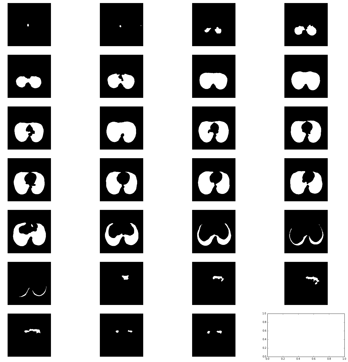
肺部区域分割

参考Candidate Generation and LUNA16 preprocessing 可实现肺部区域的分割，从而为下一步提取3d cube做准备。

def segment_lung_from_ct_scan(ct_scan):
    return np.asarray([get_segmented_lungs(slice) for slice in ct_scan])

def get_segmented_lungs(im, plot=False):

    '''
    This funtion segments the lungs from the given 2D slice.
    '''
    if plot == True:
        f, plots = plt.subplots(8, 1, figsize=(5, 40))
    '''
    Step 1: Convert into a binary image.
    '''
    binary = im < 200
    if plot == True:
        plots[0].axis('off')
        plots[0].imshow(binary, cmap=plt.cm.bone)
    '''
    Step 2: Remove the blobs connected to the border of the image.
    '''
    cleared = clear_border(binary)
    if plot == True:
        plots[1].axis('off')
        plots[1].imshow(cleared, cmap=plt.cm.bone)
    '''
    Step 3: Label the image.
    '''
    label_image = label(cleared)
    if plot == True:
        plots[2].axis('off')
        plots[2].imshow(label_image, cmap=plt.cm.bone)
    '''
    Step 4: Keep the labels with 2 largest areas.
    '''
    areas = [r.area for r in regionprops(label_image)]
    areas.sort()
    if len(areas) > 2:
        for region in regionprops(label_image):
            if region.area < areas[-2]:
                for coordinates in region.coords:
                       label_image[coordinates[0], coordinates[1]] = 0
    binary = label_image > 0
    if plot == True:
        plots[3].axis('off')
        plots[3].imshow(binary, cmap=plt.cm.bone)
    '''
    Step 5: Erosion operation with a disk of radius 2. This operation is
    seperate the lung nodules attached to the blood vessels.
    '''
    selem = disk(2)
    binary = binary_erosion(binary, selem)
    if plot == True:
        plots[4].axis('off')
        plots[4].imshow(binary, cmap=plt.cm.bone)
    '''
    Step 6: Closure operation with a disk of radius 10. This operation is
    to keep nodules attached to the lung wall.
    '''
    selem = disk(10)
    binary = binary_closing(binary, selem)
    if plot == True:
        plots[5].axis('off')
        plots[5].imshow(binary, cmap=plt.cm.bone)
    '''
    Step 7: Fill in the small holes inside the binary mask of lungs.
    '''
    edges = roberts(binary)
    binary = ndi.binary_fill_holes(edges)
    if plot == True:
        plots[6].axis('off')
        plots[6].imshow(binary, cmap=plt.cm.bone)
    '''
    Step 8: Superimpose the binary mask on the input image.
    '''
#     get_high_vals = binary == 0
#     im[get_high_vals] = 0
#     if plot == True:
#         plots[7].axis('off')
#         plots[7].imshow(im, cmap=plt.cm.bone)

    return binary

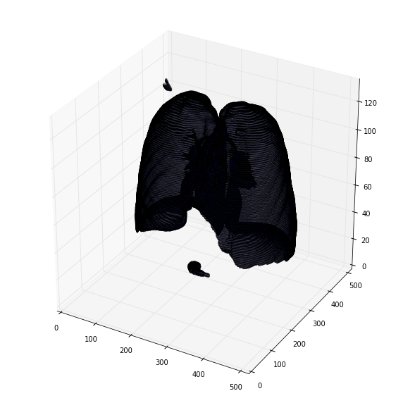
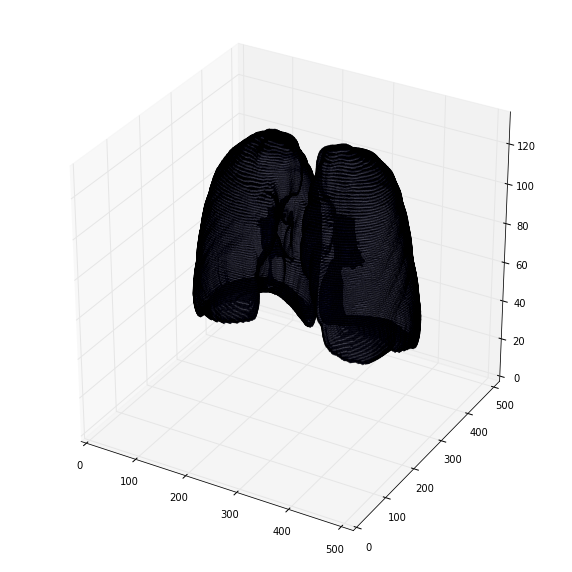
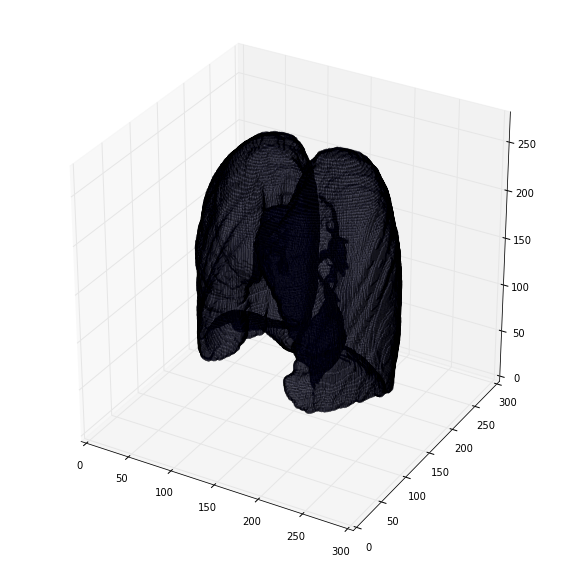
可视化3d肺部分割

def plot_3d(image, threshold=-300):
    from skimage import measure, feature

    # Position the scan upright,
    # so the head of the patient would be at the top facing the camera
    p = image.transpose(2,1,0)
    p = p[:,:,::-1]

#     print measure.marching_cubes(p, threshold)
    verts, faces, _, _= measure.marching_cubes(p, threshold)

    fig = plt.figure(figsize=(10, 10))
    ax = fig.add_subplot(111, projection='3d')

    # Fancy indexing: `verts[faces]` to generate a collection of triangles
    mesh = Poly3DCollection(verts[faces], alpha=0.1)
    face_color = [0.5, 0.5, 1]
    mesh.set_facecolor(face_color)
    ax.add_collection3d(mesh)

    ax.set_xlim(0, p.shape[0])
    ax.set_ylim(0, p.shape[1])
    ax.set_zlim(0, p.shape[2])

    plt.show()

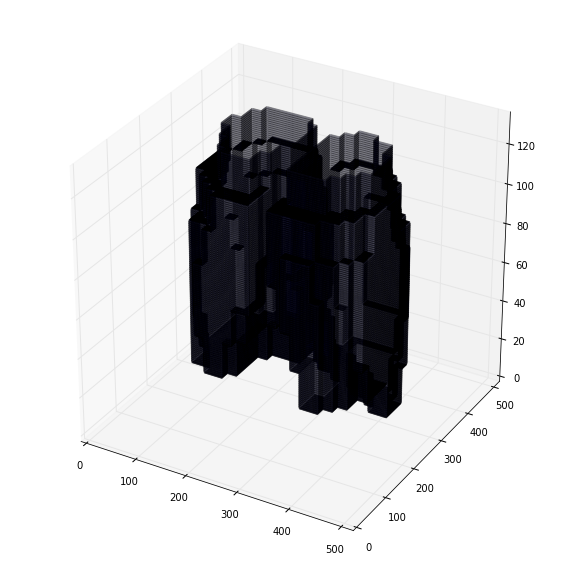
去除假阳性

selem = ball(10)
binary = binary_opening(segmented_ct_scan, selem)

label_scan = label(binary)

areas = [r.area for r in regionprops(label_scan)] # 找连通区域
areas.sort()
print areas

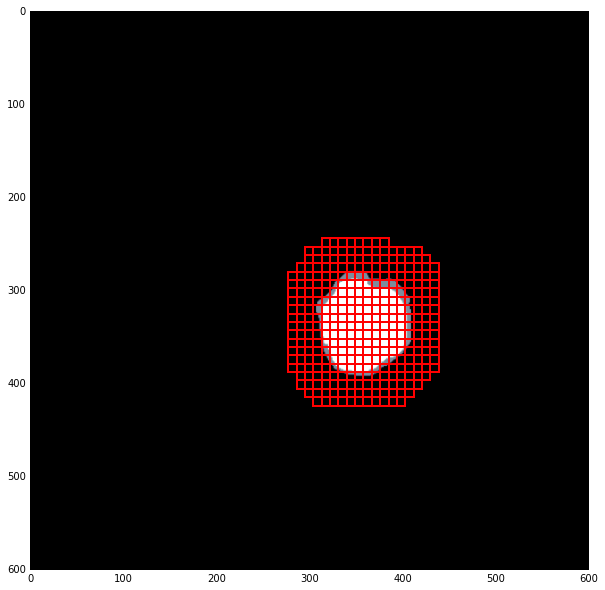
提取3d cube作为inference输入，所有cube的可视化：

差一步normalize到相同pixel spacing的过程：

检查：

模型

考虑到3d场景下做目标检测的计算量，通常分两个阶段，先筛出可疑对象，再筛掉假阳性：

Stage 1：Candidates Proposal

这个阶段的任务是尽可能找出所有可能是结节的候选（candidate）

思路1：Segmentation

例如U-net，

Merge Candidates

先腐蚀，再算连通性，再取label，每个label代表一个candidate，取mass中心，存储为csv 对照annotations.csv得到每个candidate的是TP还是FP的label，得到新的csv（最后一列为true/false的标记） 欧式距离

思路2: Object Detection

例如Faster RCNN，使用2D模型处理3D检测问题，例如每个通道代表z轴的一个slice，这样就有3个slice组成的3通道二维图像，即形如\(600\times 600 \times 3\)的image。每个通道可以是相邻的slice。

需要注意的是：考虑到肺结节的尺度比常规的自然图像中的物体要小得多，而原始的Faster RCNN使用的是16倍降采样（VGG-16Net的前四个卷积group作为feature extraction），需要通过减小降采样的方式提升ROI检测的效果。有两种思路：

1. 减少feature extractor的maxpooling层：例如删掉某个group中的maxpooling
2. 在feature extractor最后增加deconvolutional layer：例如 nn.ConvTranspose2d(1024, 1024, 4, 4, 4)会上采样4倍，这样最终是降采样4倍

另一个相伴相生的问题：标注的大小。normalize之后的结节标注可能只有1个像素大小（可能是医生标注的问题），这样即使是4倍下采样也达不到检出效果。我的方案是中心不变、扩大到8个像素。

RPN

• input：image;
• output：一系列矩形框，代表ROI，每个框都有一个objectness score，代表是物体的概率。

Stage2：False Positive Reduction

2D Resnet

可参考LUNA16 Lung Nodule Analysis

First we equalize the spacings tp 0.5mm0.5mm0.5mm using src/data_processing/equalize_spacings.py. Then we create the 96x96 patches in all three orientations using src/data_processing/create_xy_xz_yz_CARTESIUS.py. Scripts to perform this using SLURM for job management (will require some editing of paths) can be found in /scripts/create_patches/ and /scripts/rescale

• 取三个轴向的切面(patch)，根据candidate的label存储在true/false文件夹下

3d conv

由于ct是三维的，考虑使用常见的2d U-net的3d版本。

可参考：

• U-Net Segmentation Approach to Cancer Diagnosis
• 在luna上的3dconv的unet实现：Kaggle U-net
• keras 提供的conv3d：

keras.layers.convolutional.Conv3D(
    filters, # 卷积核的数目（即输出的维度）
    kernel_size, # 单个整数或由3个整数构成的list/tuple，卷积核的宽度和长度。如为单个整数，则表示在各个空间维度的相同长度。
    strides=(1, 1, 1),
    padding='valid',
    data_format=None,
    dilation_rate=(1, 1, 1),
    activation=None,
    use_bias=True,
    kernel_initializer='glorot_uniform',
    bias_initializer='zeros',
    kernel_regularizer=None,
    bias_regularizer=None,
    activity_regularizer=None,
    kernel_constraint=None,
    bias_constraint=None)

三维卷积对三维的输入进行滑动窗卷积，当使用该层作为第一层时，应提供input_shape参数。例如input_shape = (3,10,128,128)代表对10帧128*128的彩色RGB图像进行卷积。数据的通道位置仍然有data_format参数指定。

输入shape

• ‘channels_first’模式下，输入应为形如（samples，channels，input_dim1，input_dim2, input_dim3）的5D张量

• ‘channels_last’模式下，输入应为形如（samples，input_dim1，input_dim2, input_dim3，channels）的5D张量

这里的输入shape指的是函数内部实现的输入shape，而非函数接口应指定的input_shape。

评价指标

Luna官方说明：The evaluation is performed by measuring the detection sensitivity of the algorithm and the corresponding false positive rate per scan.

• TP判定（hit criterion）：candidate必须是在standard reference 中以nodule center为中心的半径R（结节直径除2）之内。hit到一个正例之后就将这个例子从表中除去，保证不重复计数。也就是说，又有第二个预测点hit到这个结节时就被忽略，不算TP。
• FP判定：在设定的半径距离内没有hit到任何reference结节.
• 忽略的情况：Candidates that are detecting irrelevant findings (see Data section in this page for definition) are ignored during the evaluation and are not considered either false positives or true positives.

最终的分数是取7个横座标点对应的纵座标（TPR）均值：

• 横座标（FPR）： 1/8, 1/4, 1/2, 1, 2, 4, and 8 FPs per scan
• 完美是1，最低是0. Most CAD systems in clinical use today have their internal threshold set to operate somewhere between 1 to 4 false positives per scan on average. Some systems allow the user to vary the threshold. To make the task more challenging, we included low false positive rates in our evaluation. This determines if a system can also identify a significant percentage of nodules with very few false alarms, as might be needed for CAD algorithms that operate more or less autonomously.

论文里关于FROC的说明：

sensitivity是关于FPR平均值的函数：

This means that the sensitivity (y) is plotted as a function of the average number of false positive markers per scan ().

• 计算FROC曲线：阈值为t，概率p≥ t则判定为结节，由此计算TPR、FPR，得到曲线上的一个点。
• 图像ID号（seriesuid）：发现结果所在的scan的名字。
• 三维坐标：浮点数（用小数点，不要用逗号）。注意：我们提供的数据的第一个体素（voxel） 的坐标是 (-128.6,-175.3,-298.3). Coordinates are given in world coordinates or millimeters. You can verify if you use the correct way of addressing voxels by checking the supplied coordinates for the example data, the locations should refer to locations that hold a nodule.
• probability : 描述为真结节的可疑程度，浮点数。通过调节对它设定的阈值来计算 FROC曲线。

Between the strings and the numbers should be a comma character. The order of the lines is irrelevant.

The following is an example result file:

seriesuid,coordX,coordY,coordZ,probability
LKDS_00001,75.5,56.0,-194.254518072,6.5243e-05
LKDS_00002,-35.5999634723,78.000078755,-13.3814265714,0.00269234
LKDS_00003,80.2837837838,198.881575673,-572.700012,0.00186072
LKDS_00004,-98.8499883785,33.6429184312,-99.7736607907,0.00035473
LKDS_00005,98.0667072477,-46.4666486536,-141.421980179,0.000256219

This file contains 8 findings (obviously way too few). There are 5 unique likelihood values. This means that there will be 5 unique thresholds that produce a distinct set of findings (each threshold discards finding below the threshold. That means there will be 5 points on the FROC curve.

It has to be noted that for the ‘false positive reduction’ challenge track, 551,065 findings (the amount of given candidates) are expected. The order of the lines is irrelevant.

本文由 Rowl1ng 创作，采用 知识共享署名4.0 国际许可协议进行许可
本站文章除注明转载/出处外，均为本站原创或翻译，转载前请务必署名
本文会经常更新，最后编辑时间为:2018-12-20 16:28:00