Choose your language :
Detectron(使用caffe2)是face book开源的的各种目标检测算法的打包(比如mask rcnn、FPN的)。 本文mask rcnn的部分基于pytorch实现的一版Detectron:Detectron.pytorch(参考了Faster R-CNN的pytorch实现),
需要安装:
- pytorch > 0.3.0
- pycocotools
- easydict
- cython
- cffi
基本概念
- IOU
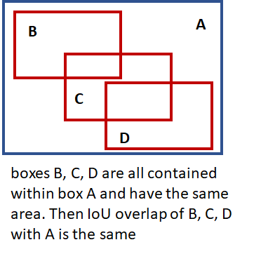
- 先明确foreground和background的概念:前景
fg(foreground)代表有物体(不管是哪个类别),背景bg(background)就是没有任何物体。
代码结构
- tools
    - train_net.py: 训练
    - test_net.py: 测试
- configs
    - 各种网络的配置文件.yml
- lib
    - core:
        - config.py: 定义了通用型rcnn可能用到的所有超参
        - test_engine.py: 整个测试流程的控制器
        - test.py
    - dataset: 原始数据IO、预处理
        - your_data.py:在这里定义你自己的数据、标注读取方式
        - roidb.py
    - roi_data:数据工厂,根据config的网络配置生成需要的各种roi、anchor等
        - loader.py
        - rpn.py: 生成RPN需要的blob
        - data_utils.py: 生成anchor
    - modeling: 各种网络插件,rpn、mask、fpn等
        - model_builder.py:构造generalized rcnn
        - ResNet.py: Resnet backbone相关
        - FPN.py:RPN with an FPN backbone
        - rpn_heads.py:RPN and Faster R-CNN outputs and losses
        - mask_rcnn_heads:Mask R-CNN outputs and losses
    - utils:小工具
数据输入
图像预处理
原项目的lib/datasets中提供了imagenet、COCO等通用数据集的调用类,如果想使用自己的数据的话就需要仿照着设计yourdata.py。几个要注意的点:
_classes:所有框的类别,比较特殊的就是__background__
# Pascal_VOC
self._classes = ('__background__',  # always index 0
                 'aeroplane', 'bicycle', 'bird', 'boat',
                 'bottle', 'bus', 'car', 'cat', 'chair',
                 'cow', 'diningtable', 'dog', 'horse',
                 'motorbike', 'person', 'pottedplant',
                 'sheep', 'sofa', 'train', 'tvmonitor')
- 关键要修改的函数就是
_load_XXX_annotation(self, index)(XXX是你的数据集的名字),要实现的功能就是给定image的index,返回所有的bounding box标注。- 返回的roidb长这样:
  return {'width': width,
      'height': height,
      'boxes': np.array(boxes),
      'gt_classes': np.array(gt_classes),
      'gt_overlaps': overlaps,
      'flipped': False, # 用于data augmentation
      'seg_areas': np.array(seg_areas)}
 # 得到roidb之后还会计算:
 'max_classes' # 和哪个class重合最大?
 'max_overlaps' # 和该class重合率[0,1]
 # 后面的采样环节会用到
- 返回的roidb长这样:
gt_overlaps:有些数据集(比如COCO)中一个bbox囊括了好几个对象,称之为crowd box,训练时需要把他们移除,移除的手段就是把它们的overlap (with all categories)设为负值(比如-1)。seg_areas: mask rcnn根据segment的区域大小排序
说一下dataset/roidb.py这个文件,里面最重要的就是combined_roidb_for_training,它是训练数据的“组装车间”,当需要同时训练多个数据集时尤为方便。通过调用每个数据集的get_roidb()方法获得各个数据集的roidb,并对相应数据集进行augmentation,这里主要是横向翻转(flipped),最后返回的是augmentation后打包在一起的roidb(前半部分是原始图像+标注,后半部分是原始图像+翻转后的标注)。
- 减去的均值是固定的\(3 \times 1\)向量(对train和test都是一样);
- Agmentation: 默认是Horizontal Flip(可以仿照加Vertically Flip)
- 控制训练时每块GPU上每个minibatch的ratio都相同:TRAIN.
ASPECT_GROUPING= True - 计算bbox regrssion \(\delta\)。需要的关键文件:utils/boxes.py
- bbox_transform_inv:通过proposal box和groundtruth box 计算bbox regrssion \(\delta\)
- MODEL.
BBOX_REG_WEIGHTS:加权用,默认是(10., 10., 5., 5.)
roi_data/loader.py中的RoiDataLoader对上面处理完的roidb“加工”成 data,主要通过get_minibatch获得某张图的一个minibatch。可以看minibatch.py的实现。首先会初始化所需blob的name list,比如FPN对应的list如下:
['roidb',
'data', # (1,3,2464,2016)
'im_info',

'rpn_labels_int32_wide_fpn2', # (1,3,752,752)
'rpn_labels_int32_wide_fpn3', # (1,3,376,376)
'rpn_labels_int32_wide_fpn4',  # (1,3,188,188)
'rpn_labels_int32_wide_fpn5', # (1,3,94,94)
'rpn_labels_int32_wide_fpn6', # (1,3,47,47)

'rpn_bbox_targets_wide_fpn2', # (1,12,752,752)
'rpn_bbox_targets_wide_fpn3',
'rpn_bbox_targets_wide_fpn6',
'rpn_bbox_targets_wide_fpn4',
'rpn_bbox_targets_wide_fpn5',

'rpn_bbox_outside_weights_wide_fpn2', # (1,12,752,752)
'rpn_bbox_outside_weights_wide_fpn3',
'rpn_bbox_outside_weights_wide_fpn4',
'rpn_bbox_outside_weights_wide_fpn5',
'rpn_bbox_outside_weights_wide_fpn6',

'rpn_bbox_inside_weights_wide_fpn6',
'rpn_bbox_inside_weights_wide_fpn5',
'rpn_bbox_inside_weights_wide_fpn4',
'rpn_bbox_inside_weights_wide_fpn3',
'rpn_bbox_inside_weights_wide_fpn2'] # (1,12,752,752)
在获得list后,使用roi_data/rpn.py的add_rpn_blobs来填上对应的blob。_get_rpn_blobs的流程:
- 生成anchor
- TRAIN.
RPN_STRADDLE_THRESH:筛除超出image范围的RPN anchor,默认是0. - 计算anchor label: positive:label=1; negative:label=0;don’t care: label=-1
- 计算anchor和gt box的overlap
- Fg label(positive):和每个gt重合率最大的那个anchor;超过TRAIN.
RPN_POSITIVE_OVERLAP的anchor
- Fg label(positive):和每个gt重合率最大的那个anchor;超过TRAIN.
- 控制数量,采样positive 和 nagative label,超过的将label设为-1
- fg/正样本:
- 总数 =
TRAIN.FG_FRACTION*TRAIN.BATCH_SIZE_PER_IM - 条件:>
TRAIN.FG_THRESH,随机选择达到条件的fg,数量<=总数:fg_inds = np.where(max_overlaps>= cfg.TRAIN.FG_THRESH)[0]
- 总数 =
- bg/负样本:
- 总数 =
TRAIN.BATCH_SIZE_PER_IM- 正样本总数 - 条件:[
BG_THRESH_LO,BG_THRESH_HI)
- 总数 =
- fg/正样本:
- 计算anchor和gt box的overlap
- bbox regression loss:loss(x) = weight_outside * L(weight_inside * x)
- bbox_inside_weights: bbox regression只用positive example来训,所以只需把positive的weight设为1.0,其他设为0即可(只有那些分类正确了的box才能参与,分类错误的直接不考虑了)
- bbox_outside_weights: bbox regression loss是对minibatch中的图片数取平均,
着部分的逻辑可以看作是确保bg和fg的样本数量之和是一个常数。万一找到的bg样本太少,就随机重复一些来填补que Bbox regression loss has the form: # Inside weights allow us to set zero loss on an element-wise basis # Bbox regression is only trained on positive examples so we set their # weights to 1.0 (or otherwise if config is different) and 0 otherwise
代码实现上:使用了mask array将for循环操作转化成了矩阵乘法。mask array标注了每个anchor的正确物体类别。
正负采样
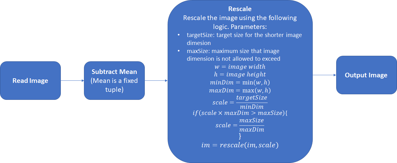
- 考虑到一块gpu的显存有限,我们往往需要将图像rescale的一定大小。
targetSize和maxSize默认是 600 和 1000 ,根据显存大小和图片大小来设计就好(比如最长边限制在2100或者短边是1700的时候一块gpu只能跑一个sample)。TRAIN.SCALES:一个list,默认是[600,],如果有多个值,在采样的时候是随机分配给image的:np.random.randint(0, high=len(cfg.TRAIN.SCALES), size=num_images)
关键文件: roi_data/fast_rcnn.py
- _sample_rois:随机采样fg/bg examples,控制数量的方法和之前一样
Rescale的基本逻辑如下图:
这一步在决定使用的anchor size时一定要考虑进去,github上有人写过基于自己数据的分析脚本,基本思路是还原rescale的过程,分析rescale factor,估计一下roi的大小,从而决定anchor size。
计算所有ROI和所有ground truth的max overlap,从而判断是fg还是bg。这里用到了两个参数:
TRAIN.FG_THRESH:用来判断fg ROI(default:0.5)TRAIN.BG_THRESH_LO~TRAIN.BG_THRESH_HI:这个区间的是bg ROI。(default 0.1, 0.5 respectively)
这样的设计可以看作是 “hard negative mining” ,用来给classifier投喂更难的bg样本。
输入:
- proposal layer得到的ROIs
- ground truth information
输出:
- 选出满足overlap要求的bg、fg的ROI。
- 每个roi针对不同类别的regression coefficients。
Parameters:
TRAIN.BATCH_SIZE: (default 128) 所选fg和bg box的最大数量.TRAIN.FG_FRACTION: (default 0.25). fg box 不能超过 BATCH_SIZE*FG_FRACTION
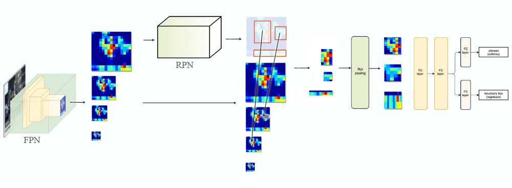
Generalized RCNN结构
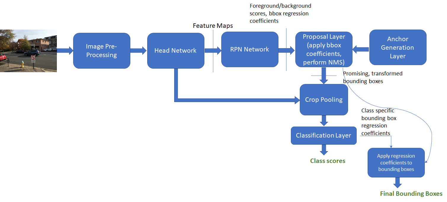
R-CNN包括三种主要网络:
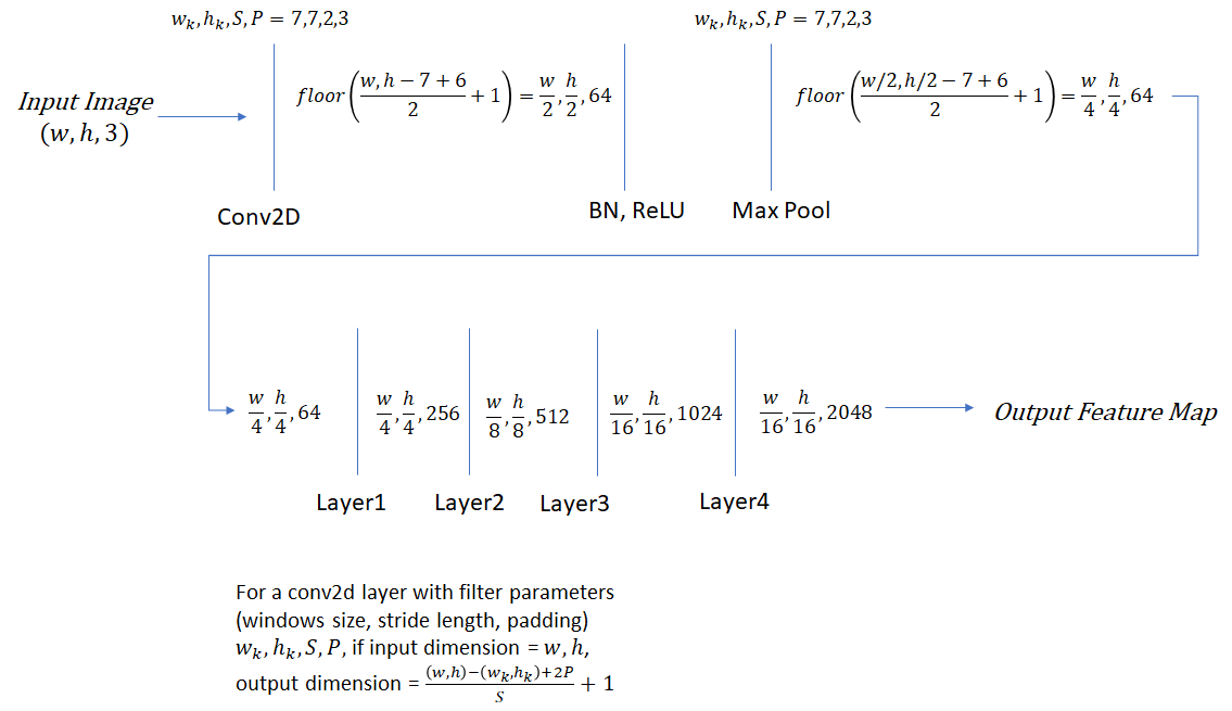
- Head:输入(w,h,3)生成feature map,降采样了16倍; w和h是预处理以后的图片大小哦
- Region Proposal Network (RPN):基于feature map,预测ROI;
Crop Pooling:从feature map中crop相应位置
- Classification Network:对crop出的区域进行分类。
在pytorch版Detectron中,medeling/model_builder.py中的generalized_rcnn将FPN、fast rcnn、mask rcnn作为“插件”,通过config文件中控制“插拔”。
MODEL:
  TYPE: generalized_rcnn
  CONV_BODY: FPN.fpn_ResNet50_conv5_body # backbone
  FASTER_RCNN: True # RPN ON
  MASK_ON: True # 使用mask支线:mask rcnn除了box head,还有一个mask head。
在Detectron的实现里,可以像上面这样在config文件中灵活选择使用的backbone(比如conv body使用Res50_conv4,roi_mask_head和box head共同使用fcn_head)。代码模块划分:
Conv_Body对应下图中的head: 输入im_data,返回blob_convRPN对应下图中的Region Proposal Network: loss_rpn_cls + loss_rpn_bbox # 输入blob_conv,返回rpn_ret;BBOX_Branch:loss_rcnn_cls + loss_rcnn_bboxBox_Head对应下图中的Generate Grid Points Sample Feature Maps + Layer4 # 输入conv_body, rpn_ret返回box_feat- 通过FAST_RCNN.ROI_BOX_HEAD设置
Box_Outs对应下图中的cls_score_net + bbx_pred_net# 输入box_feat, 返回cls_score, bbox_pred, 计算loss_cls, loss_bbox
Mask_Branch: loss_rcnn_mask- Mask_Head# 输入blob_conv, rpn_net, 返回mask_feat
- 通过MRCNN.ROI_MASK_HEAD设置
- Mask_Outs# 输入mask_feat,返回mask_pred
- Mask_Head# 输入blob_conv, rpn_net, 返回mask_feat

先来看看Head怎么得到feature map。拿VGG16作为backbone来举例的话,一个完整的VGG16网络长这样:

其中红色部分就是下采样的时刻。原始论文里使用VGG16,因为提feature map只用了最后一次max pooling前面的部分,所以留下来的四次pooling总共下采样是16倍。得到的feature map长这样:

最终的feature映射回原图的话大概长这样:

有了feature map以后,开始走RCNN的主体流程:
Backbone
在初始化generalized rcnn时,首先要选择backbone(也许可以意译为“骨干网”)。通过cfg.MODEL.CONV_BODY即可选择backbone:
self.Conv_Body = get_func(cfg.MODEL.CONV_BODY)() # 如果是FPN,会在这一步直接基于backbone完成FPN的构造
Resnet
Resnet.py打包了各种resnet的backbone,比如ResNet50_conv5_body:
def ResNet50_conv5_body():
    return ResNet_convX_body((3, 4, 6, 3)) # block_counts: 分别对应res2、res3、res4、res5
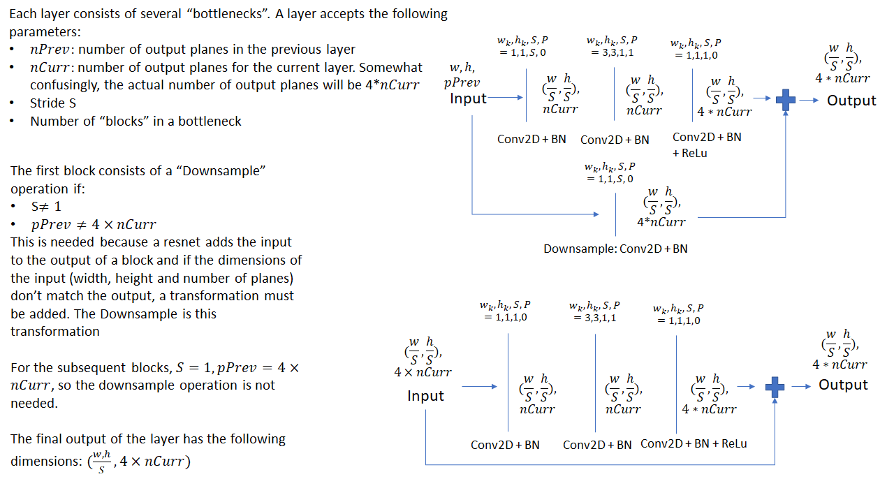
Resnet中的Bottleneck:
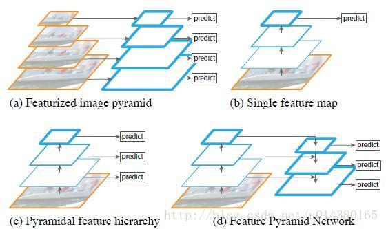
FPN
可以选择是否用于RoI transform,是否用于RPN:
- feature extraction:fpn.py中的fpn类将backbone“加工”为FPN。比如当config里的CONV_BODY: FPN.fpn_ResNet50_conv5_body,实际要做的就是先初始化Resnet.ResNet50_conv5_body,再交给fpn得到fpn_ResNet50_conv5_body。
- RPN with FPN backbone: 如果rpn使用FPN,那么FPN的每个level都会做RPN,生成相应大小的anchor,返回相应的cls_score和bbox_pred。rpn_heads,FPN.fpn_rpn_outputs
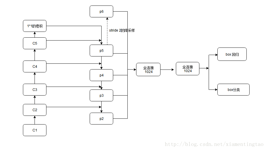

 可以看到降采样从P5到P2是(1. / 32., 1. / 16., 1. / 8., 1. / 4.)
选择:
FPN.EXTRA_CONV_LEVELS:可以选择是否加上P6,即最上层stride2的降采样后的Output,这样降采样就还加上 1. / 64.- P2Only:选择是否只使用P2的Output
# FPN is enabled if True
__C.FPN.FPN_ON = False

# Channel dimension of the FPN feature levels
__C.FPN.DIM = 256

# Initialize the lateral connections to output zero if True
__C.FPN.ZERO_INIT_LATERAL = False

# Stride of the coarsest FPN level
# This is needed so the input can be padded properly
__C.FPN.COARSEST_STRIDE = 32

#
# FPN may be used for just RPN, just object detection, or both
#

# Use FPN for RoI transform for object detection if True
__C.FPN.MULTILEVEL_ROIS = False
# Hyperparameters for the RoI-to-FPN level mapping heuristic
__C.FPN.ROI_CANONICAL_SCALE = 224  # s0
__C.FPN.ROI_CANONICAL_LEVEL = 4  # k0: where s0 maps to
# Coarsest level of the FPN pyramid
__C.FPN.ROI_MAX_LEVEL = 5
# Finest level of the FPN pyramid
__C.FPN.ROI_MIN_LEVEL = 2

# Use FPN for RPN if True
__C.FPN.MULTILEVEL_RPN = False
# Coarsest level of the FPN pyramid
__C.FPN.RPN_MAX_LEVEL = 6
# Finest level of the FPN pyramid
__C.FPN.RPN_MIN_LEVEL = 2
# FPN RPN anchor aspect ratios
__C.FPN.RPN_ASPECT_RATIOS = (0.5, 1, 2)
# RPN anchors start at this size on RPN_MIN_LEVEL
# The anchor size doubled each level after that
# With a default of 32 and levels 2 to 6, we get anchor sizes of 32 to 512
__C.FPN.RPN_ANCHOR_START_SIZE = 32
# Use extra FPN levels, as done in the RetinaNet paper
__C.FPN.EXTRA_CONV_LEVELS = False
1. Anchor Generation Layer
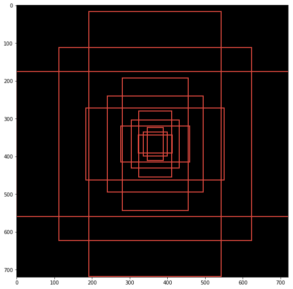
第一步就是生成anchor(lib/modeling/generate_anchors.py),这里的anchor亦可理解为bounding box。Anchor Generation Layer的任务是对feature map上的每个点都计算若干anchor。而RPN的任务就是判断哪些是好的anchor(包含gt对象)并计算regression coefficients(优化anchor的位置,更好地贴合object):
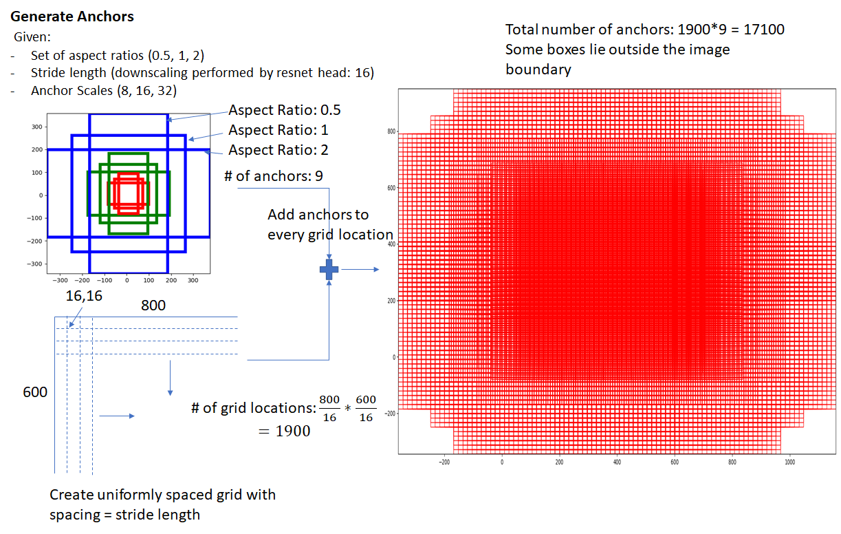
- 三种颜色分别代表128x128, 256x256, 512x512
- 每种颜色的三个框分别代表比例1:1, 1:2 and 2:1
- 每种颜色的三个框的面积是差不多的,因此,可以说最大识别框的面积是 512 x 512
anchor是RPN的windows的大小,在feature map的每一个位置使用不同尺度和长宽比的window提取特征。原论文描述为“a pyramid of regression references”。
对应到代码上:比如ANCHOR_SCALES是[4, 8, 16, 32],ANCHOR_RATIOS默认是[0.5,1,2]。
#imagenet
args.set_cfgs = ['ANCHOR_SCALES', '[4, 8, 16, 32]', 'ANCHOR_RATIOS', '[0.5,1,2]', 'MAX_NUM_GT_BOXES', '30']
但是并不是越多越好,要控制在一定的数量,理由是:
- anchors多了就会造成faster RCNN的时间复杂度提高,anchors多的最极端情况就是overfeats中sliding windows。
- 使用多尺度的anchors未必全部对scale-invariant property都有贡献
所以,在使用自己的数据的时候,统计一下gorund truth框的大小(注意考虑预处理rescale的系数),确定大小范围还是很有必要的。
2. Region Proposal Layer
前一步生成anchor得到的是dense candidate region,rpn根据region是fg的概率来对所有region排序。
Region Proposal Layer的两个任务就是:
rpn_cls_score:判断anchor是前景还是背景rpn_bbox_pred:根据regression coefficient调整anchor的位置、长宽,从而改进anchor,比如让它们更贴合物体边界。
2.1 Region Proposal Network
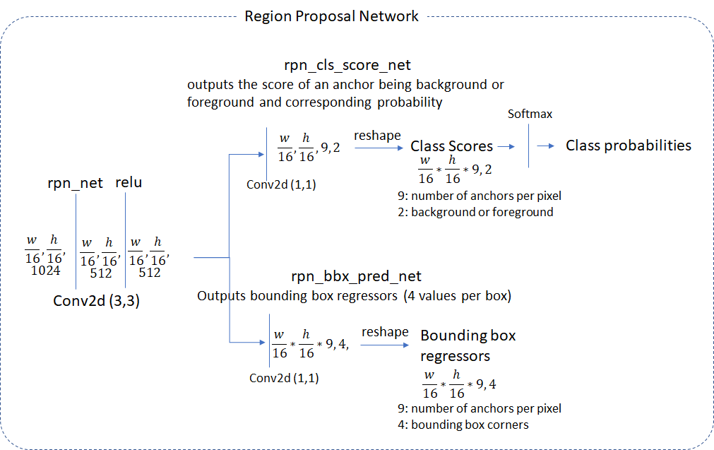
值得注意的是,这里的anchor是以降采样16倍的卷积网(called rpn_net in code)得到的feature map为基础的。
rpn_net的输出通过两个 (1,1)核的卷积网,从而产生bg/fg的class scores以及对应的bbox的regression coefficient。head network使用的stride和生成anchor使用的stride一致,所以anchor和rpn产生的信息是一一对应的,即 number of anchor boxes = number of class scores = number of bounding box regression coefficients = \(\frac{w}{16}\times\frac{h}{16}\times9\)
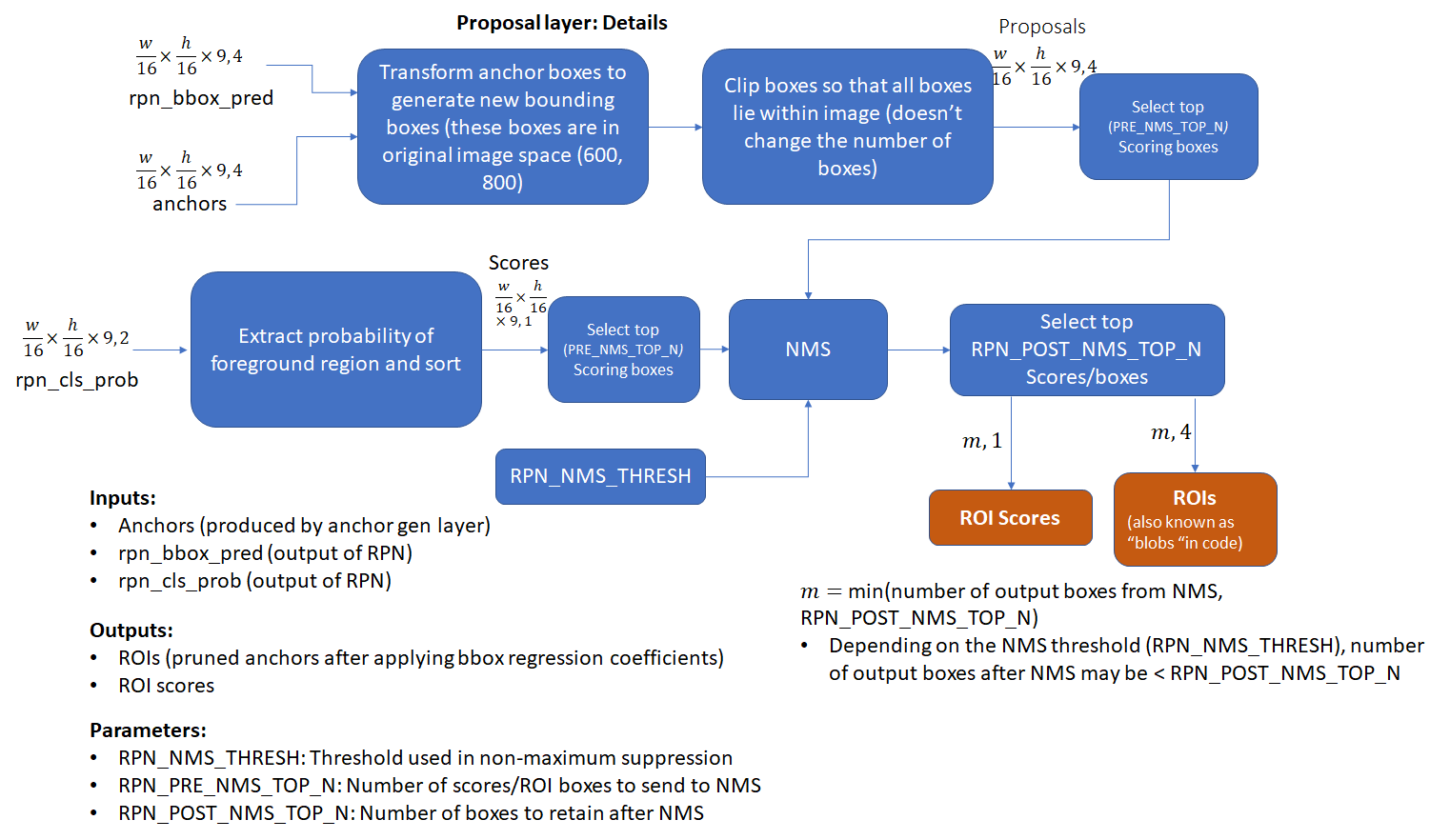
2.2 Proposal Layer
proposal layer基于anchor generation layer得到的anchor,使用nms(基于fg的score)来筛除多余的anchor。此外,它还负责将RPN得到的regression coefficients应用到对应的anchor上,从而得到transformed bbox。
2.3 Anchor Target Layer
anchor target layer 的目标在于选择可靠的anchor来训练RPN:
- 区分bg/fg区域,
- 为fg box生成好的bbox regression coefficients
首先看一看RPN loss的计算过程,了解其中用到的信息有助于理解Anchor Target Layer的流程。
计算RPN loss:
前面提到RPN的目标是得到好的bbox,而达到这个目的的必经之路就是:1. 学会判断一个anchor是fg/bg;2. 计算regression coefficients来修正fg anchor的位置、宽、高,从而更好地贴合对象。因此, RPN Loss的计算就是为了优化以上两点:
\[RPN Loss = \text{Classification Loss} + \text{Bounding Box Regression Loss}\]- Classification Loss: cross_entropy(predicted _class, actual_class)
- Bounding Box Regression Loss:\(L_{loc} = \sum_{u \in {\text{all foreground anchors}}}l_u\)
由于bg的anchor没有可以回归的target bbox,这里只对所有fg的regression loss求和。计算某个bg anchor的regression loss的方法:
\(l_u = \sum_{i \in {x,y,w,h}}smooth_{L1}(u_i(predicted)-u_i(target))\)x y w h分别对应bbox的左上角坐标和长宽。 体现在代码里:
loss_rpn_bbox = net_utils.smooth_l1_loss(
        rpn_bbox_pred, rpn_bbox_targets, rpn_bbox_inside_weights, rpn_bbox_outside_weights,
        beta=1./9)
smooth L1 function: \(smooth_{L1}(x) = \begin{cases} \frac{\sigma^2x^2}{2} & \lVert x \rVert < \frac{1}{\sigma^2} \\ \lVert x \rVert - \frac{0.5}{\sigma^2} & otherwise\end{cases}\)
这里的\(\sigma\)是随机选的。
因此,为了计算loss我们需要计算以下数值:
- Class labels (background or foreground) and scores for the anchor boxes
- Target regression coefficients for the foreground anchor boxes
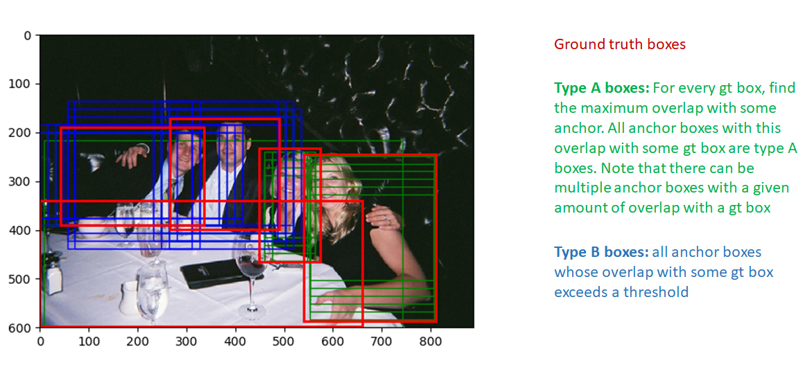
现在我们通过anchor target layer的实现来看看这些值计算过程: 首先我们选择在image范围内的anchor box,然后通过计算所有anchor box和所有gt box的IOU来选取好的fg box。 使用overlap信息,有两种类型的box将被标记为fg:
- type A: 对每个gt box,所有和它有最大iou overlap的fg box
- type B: 和某些gt box最大overlap超过一定阈值的anchor box
体现在代码里:
# Fg label: for each gt use anchors with highest overlap
# (including ties)
labels[anchors_with_max_overlap] = 1
# Fg label: above threshold IOU
labels[anchor_to_gt_max >= cfg.TRAIN.RPN_POSITIVE_OVERLAP] = 1
需要注意的是和某gt box的overlap超过一定阈值的anchor box才被认为是fg box。这是为了避免让RPN学习注定失败的任务:要学习的box的regression coefficients和最佳匹配的gt box隔得太远。同理,overlap小于某阈值的box即为bg box。需要注意的是,fg/bg并不是“非黑即白”,而是有“don’t care”这单独的一类,用来标识既不是fg也不是bg的box,这些框也就不在loss的计算范围中。同时,“don’t care”也用来约束fg和bg的总数和比例,比如多余的fg随机标为“don’t care”。
There are two additional thresholds related to the total number of background and foreground boxes we want to achieve and the fraction of this number that should be foreground. If the number of foreground boxes that pass the test exceeds the threshold, we randomly mark the excess foreground boxes to “don’t care”. Similar logic is applied to the background boxes.
Next, we compute bounding box regression coefficients between the foreground boxes and the corresponding ground truth box with maximum overlap. This is easy and one just needs to follow the formula to calculate the regression coefficients.
This concludes our discussion of the anchor target layer. To recap, let’s list the parameters and input/output for this layer:
一些相关参数:
TRAIN.RPN_POSITIVE_OVERLAP: 用来筛选fg box的阈值(Default: 0.7)TRAIN.RPN_NEGATIVE_OVERLAP: 用来筛选bg box的阈值(Default: 0.3)。这样一来,和ground truth的overlap在0.3~0.7就是“don’t care”。TRAIN.RPN_BATCHSIZE: fg和bg anchor的总数 (default: 256)TRAIN.RPN_FG_FRACTION: batch size中fg的比例 (default: 0.5)。如果fg数量超过 TRAIN.RPN_BATCHSIZE$\times$ TRAIN.RPN_FG_FRACTION, 超过的部分 (根据索引随机选择) 就被标为 “don’t care”.
输入:
- RPN Network Outputs (predicted foreground/background class labels, regression coefficients)
- Anchor boxes (generated by the anchor generation layer)
- Ground truth boxes
输出:
- Good foreground/background boxes and associated class labels
- Target regression coefficients
2.4 Proposal Target Layer
前面提到proposal layer负责产生ROI list,而Proposal Target Layer负责从这个list中选出可信的ROI。这些ROI将经过 crop pooling从feature map中crop出相应区域,传给后面的classification layer(head_to_tail).
和anchor target layer相似,Proposal Target Layer的重要性在于:如果这一步不能选出好的候选(和ground truth 尽可能重合),后面的classification也是“巧妇难为无米之炊”。
具体来说:在得到了proposal layer的roi之后,对每个ROI,计算和每个ground truth的最大重合率,这样就把ROI划分成了bg和fg:
- fg ROI:和每个ground truth的重合都超过了阈值(
TRAIN.FG_THRESH, default: 0.5) - bg ROI:最大重合率阈值在
TRAIN.BG_THRESH_LO和TRAIN.BG_THRESH_HI(default 0.1, 0.5 respectively)之间。
这个过程可以理解为一种“hard negative mining”:把更难的bg 样本输送给classifier。
在这之后,要计算每个ROI和与它最接近的ground truth box之间的regression target(这一步也包含bg ROI,因为这些ROI也有重合的ground truth box)。所有类别的regression target如下:
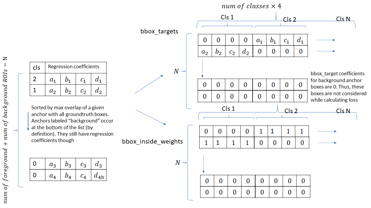
这个bbox_inside_weights起一个mask的作用,只有对分类正确的fg roi才是1,而所有bg都是0,这样就只计算fg的loss,不管bg的,但是算分类loss的时候还是都考虑。
输入:
- ROIs produced by the proposal layer
- ground truth information
输出:
- Selected foreground and background ROIs that meet overlap criteria.
- Class specific target regression coefficients for the ROIs
参数:
- TRAIN.FG_THRESH: (default: 0.5) Used to select foreground ROIs. ROIs whose max overlap with a ground truth box exceeds FG_THRESH are marked foreground
- TRAIN.BG_THRESH_HI: (default 0.5)
- TRAIN.BG_THRESH_LO: (default 0.1) These two thresholds are used to select background ROIs. ROIs whose max overlap falls between BG_THRESH_HI and BG_THRESH_LO are marked background
- TRAIN.BATCH_SIZE: (default 128) Maximum number of foreground and background boxes selected.
- TRAIN.FG_FRACTION: (default 0.25). Number of foreground boxes can’t exceed BATCH_SIZE*FG_FRACTION
3.Crop Pooling layer
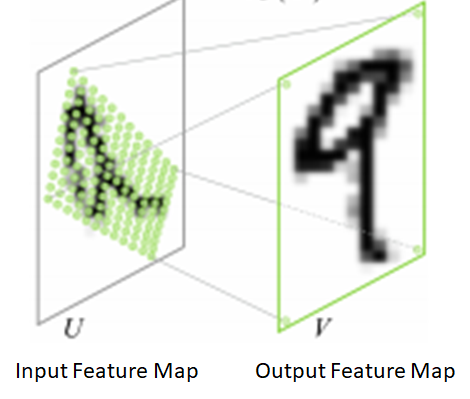
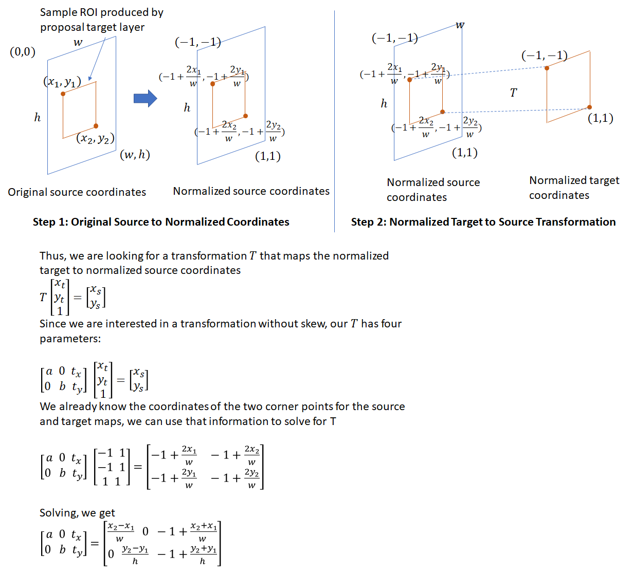
有了Proposal Target Layer计算的ROI的包含class label、regression coefficients的regression target,下一步就是从从feature map中提取ROI对应区域。所抽取的区域将参与tail部分的网络,并最终输出每个ROI对应的class probability distribution 和 regression coefficients,这也就是Crop Pooling layer的任务。其关键思想可以参考Spatial Transformation Networks,其目标是提供一个warping function( a \(2\times 3\) affine transformation matrix):将输入的feature map映射到warped feature map,如下图:
包括两步:
- \(\begin{bmatrix} x_i^s \\ y_i^s \end{bmatrix} = \begin{bmatrix} \theta_{11} & \theta_{12} & \theta_{13} \\ \theta_{21} & \theta_{22} & \theta_{23} \end{bmatrix}\begin{bmatrix} x_i^t \\ y_i^t \\ 1\end{bmatrix}\). 这里\(x_i^s, y_i^s, x_i^t, y_i^t\) 是 height/width normalized coordinates (similar to the texture coordinates used in graphics), 所以\(-1 \leq x_i^s, y_i^s, x_i^t, y_i^t \leq 1\).
- 第二步, 输入的source map经过source坐标的采样输出destination map。在这一步中,每个 \((x_i^s, y_i^s)\)坐标都定义了输入中sampling kernel(for example bi-linear sampling kernel) 所应用的空间位置,从而得到输出的feature map中每个pixel的值
不同的pooling模式:
- crop
- align
主要用到Pytorch的torch.nn.functional.affine_grid 和torch.nn.functional.grid_sample
crop pooling的步骤:
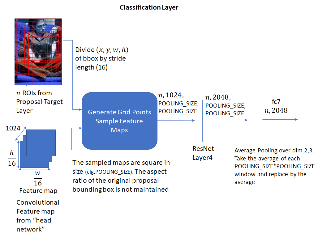
- ROI坐标 $\div$ head网络下采样的倍数(也就是stride)。需要特别指出的是:proposal target layer给出的ROI坐标是原图尺度上的(默认800$\times$600),因此映射到feature map之前要先除stride(默认是16,前面解释过)。
- affine transformation matrix(仿射变换矩阵)
- 最关键的一点在于后面的分类网接收的是固定大小输入,因此这一步需要把矩形窗
4.Classification Layer
crop pooling layer基于proposal target layer生成的ROI boxes和“head” network的convolutional feature maps,生成square feature maps。 feature maps接下来通过ResNet的layer4、沿着spatial维的average pooling,结果(called “fc7” in code) 是每个ROI的一维特征向量。过程如下:
fc之后得到的一维特征向量被送到两个全连接网络中:bbox_pred_net and cls_score_net
cls_score_net:生成roi每个类别的score(softmax之后就是概率了)bbox_pred_net:结合两者得到最终的bbox坐标- class specific bounding box regression coefficients
- 原来proposal target layer生成的 bbox 坐标
过程如下:
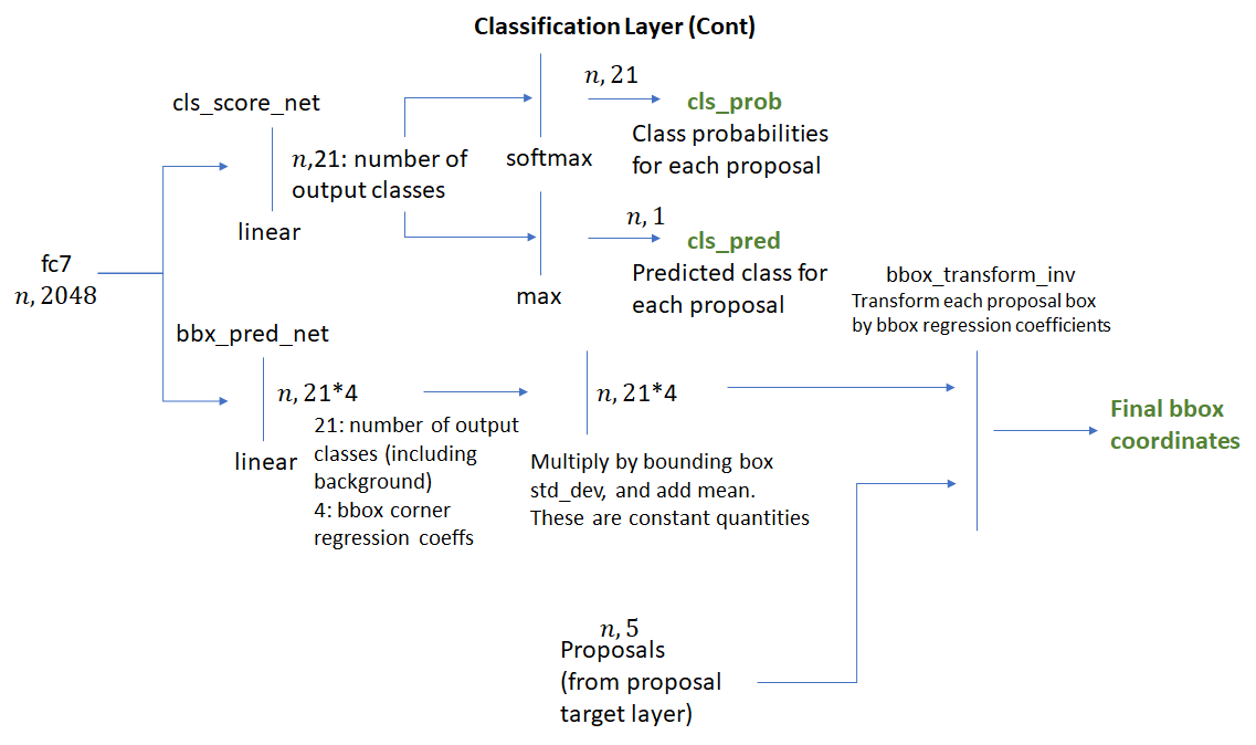
有意思的是,训练classification layer得到的loss也会反向传播给RPN。这是因为用来做crop pooling的ROI box坐标不仅是RPN产生的 regression coefficients应用到anchor box上的结果,其本身也是网络输出。因此,在反传的时候,误差会通过roi pooling layer传播到RPN layer。好在crop pooling在Pytorch中有内部实现,省去了计算梯度的麻烦。
计算 Classification Layer Loss
这个阶段要把不同物体的标签考虑进来了,所以是一个多分类问题。使用交叉熵计算分类Loss:
这个阶段依然要计算bounding box regression loss,和前面的R区别PN的区别在于:
- RPN的是为了让bbox更紧凑地贴合物体。 anchor target layer算得的target regression coefficients需要将roi box和离它最近的ground truth bbox对齐。
- classification layer中的是针对各个类别的。也就是说,对每个roi、每个类别都会生成一套coefficient。只有那些分类正确了的box才能参与,分类错误的直接不考虑了。
代码实现上:使用了mask array将for循环操作转化成了矩阵乘法。mask array标注了每个anchor的正确物体类别。
考虑到计算Classification Layer Loss和计算RPN Loss十分相似,在此先讲。
\[\text{Classification Layer Loss} = \text{Classification Loss} + \text{Bounding Box Regression Loss}\]classification layer和RPN的关键区别是:RPN处理的是bg/fg的问题,classification layer处理的是所有的物体分类(加上bg)
- classification loss:cross entropy loss with the true object class and predicted class score as the parameters. 计算过程如下:
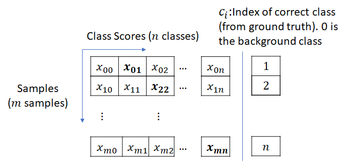

- bounding box regression loss:和RPN的时候类似,除了现在 regression coefficients是针对class的. 也就是说,会针对每个object类型计算 regression coefficients. 显然,对某anchor box来说,最大重合的gt box所属的类别算得的 target regression coefficients 才是可用的。在计算loss时,会以mask array的形式标记出每个anchor box的正确class。分类错误的其余class 的 regression coefficients 就被忽略了. This mask array allows the computation of loss to be a matrix multiplication as opposed to requiring a for-each loop.
因此计算Classification Layer Loss需要以下3个数值:
- 预测的class label和bbox regression coefficients (these are outputs of the classification network)
- 每个 anchor box的class labels
- Target bounding box regression coefficients
Mask-RCNN
mask rcnn里默认的mask head是conv层,也可以通过MRCNN.USE_FC_OUTPUT设置使用FC层。
- 做分割的话,关键是roi pooling时候的对齐问题,mask rcnn提出roi align face++提出precise roi pooling,使用$x/16$而不是$[x/16]$,使用bilinear interpolation
- 分隔开分割和分类两个任务,mask rcnn中对每个类别都会生成一个mask,或者是class-agnostic的实验中,不管类别直接生成mask,效果都不错
- [关于mask rcnn实现的讨论][241],kaggle上也有一个做医疗图像的demo
Inference
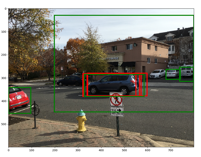
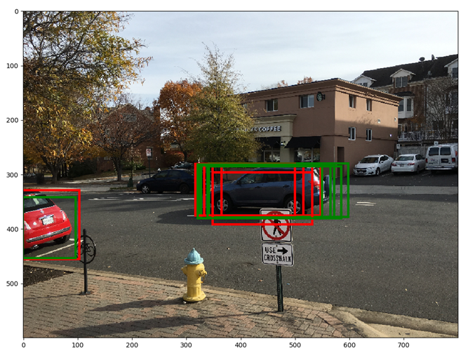 The red boxes show the top 6 anchors ranked by score. Green boxes show the anchor boxes after applying the regression parameters computed by the RPN network. The green boxes appear to fit the underlying object more tightly. Note that after applying the regression parameters, a rectangle remains a rectangle, i.e., there is no shear. Also note the significant overlap between rectangles. This redundancy is addressed by applying non-maxima suppression
 Red boxes show the top 5 bounding boxes before NMS, green boxes show the top 5 boxes after NMS. By suppressing overlapping boxes, other boxes (lower in the scores list) get a chance to move up
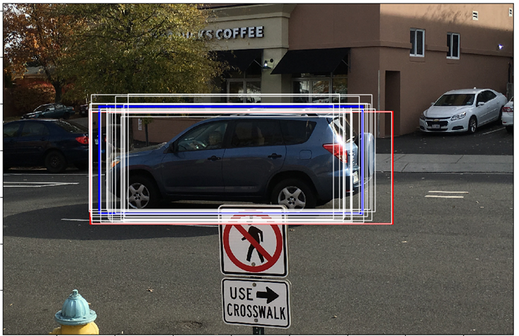 From the final classification scores array (dim: n, 21), we select the column corresponding to a certain foreground object, say car. Then, we select the row corresponding to the max score in this array. This row corresponds to the proposal that is most likely to be a car. Let the index of this row be car_score_max_idx Now, let the array of final bounding box coordinates (after applying the regression coefficients) be bboxes (dim: n,21*4). From this array, we select the row corresponding to car_score_max_idx. We expect that the bounding box corresponding to the car column should fit the car in the test image better than the other bounding boxes (which correspond to the wrong object classes). This is indeed the case. The red box corresponds to the original proposal box, the blue box is the calculated bounding box for the car class and the white boxes correspond to the other (incorrect) foreground classes. It can be seen that the blue box fits the actual car better than the other boxes.
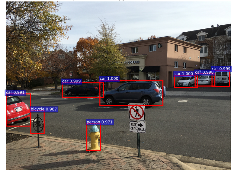
For showing the final classification results, we apply another round of NMS and apply an object detection threshold to the class scores. We then draw all transformed bounding boxes corresponding to the ROIs that meet the detection threshold. The result is shown below.
Appendix
非极大值抑制(non-maximum suppression,nms)

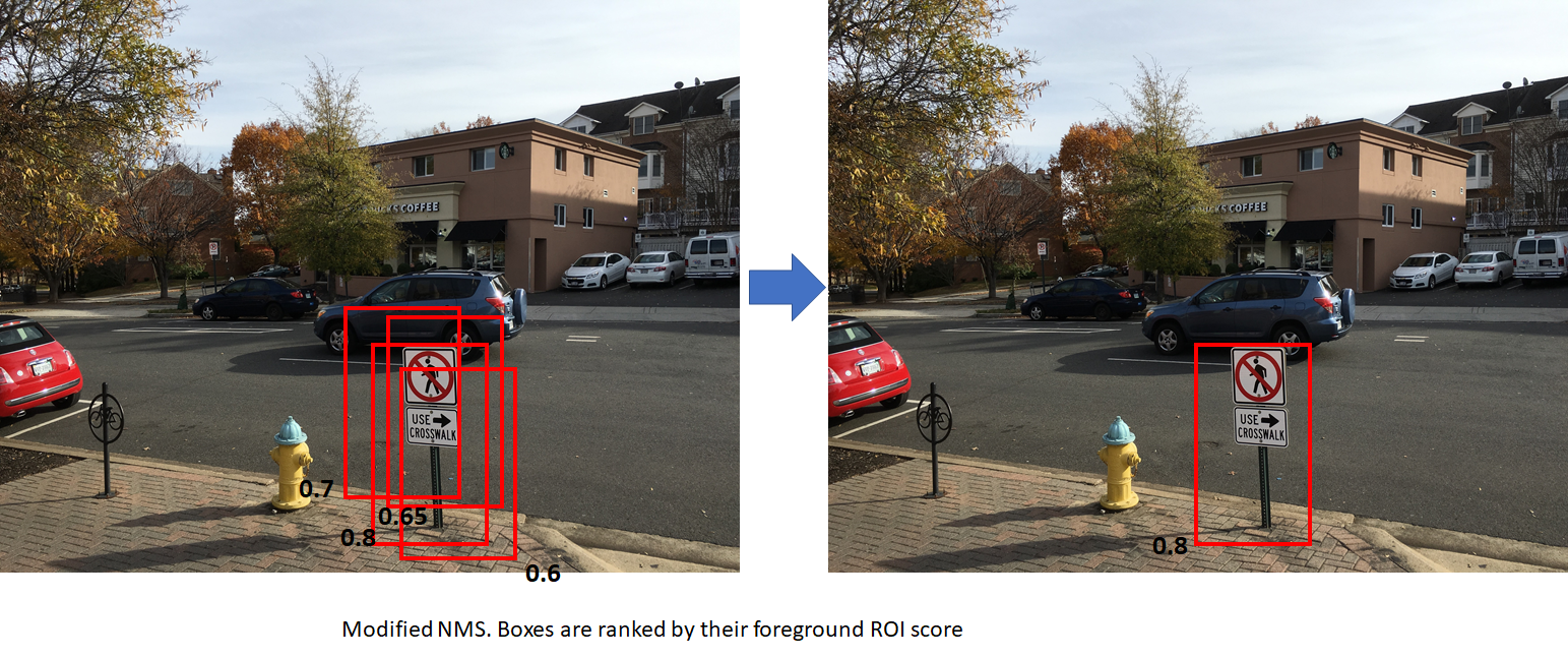
上图左边的黑色数字代表fg的概率
- standard NMS (boxes are ranked by y coordinate of bottom right corner). This results in the box with a lower score being retained. The second figure uses modified NMS (boxes are ranked by foreground scores).
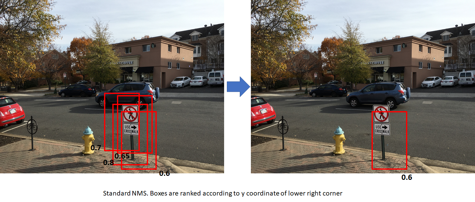
- This results in the box with the highest foreground score being retained, which is more desirable. In both cases, the overlap between the boxes is assumed to be higher than the NMS overlap threhold.
讲nms(non-maximum suppression)的文章
针对小物体
每个小红点之间就是16像素的间隔了,如果要检测特别细小的物体,这么大的下采样就很危险了。于是,为了尽量不破坏细小物体的清晰度,参考github上关于检测微小物体的讨论,我尝试了两种方案:
1. 降低下采样倍数
为了方便实验,我给网络增加了一个参数downsample,用来控制下采样倍数,相应地调整网络结构:
parser.add_argument('--downsample', dest='downsample_rate',
                  help='downsample',
                  default=16, type=int) # 原网络默认16倍
需要注意的是:
- 一旦改变下采样,同时还要改变feature_stride和spatial_scale。否则预测框框就变成了边缘的线条(同时loss_rpn_cls奇高)。比如VGG16(降采样8倍):
- __C.feat_stride’: 8”
- self.spatial_scale to (1/8)
- vgg16尝试4倍下采样:去掉了stage5的卷积,保障输入图像最短边在1200
2. 切割原图
- 训练数据切patch:将原图切分为四等份再训练,保障大部分图的清晰度不被压缩。这样一来,标注也要做调整:
- 一种方式是重新生成新的子图标注,新写一个yourdata.py;
- 另一种偷懒方式则是修改 yourdata.py的
_load_XXX_anotation(self, index),使得读入每个子图,返回的也是每个子图的所有标注框。
- 测试数据为原图,沿用原来的数据读入方式即可。
训练:Minibatch SGD
Linear Scaling Rule: When the minibatch size ismultiplied by k, multiply the learning rate by k.
warmup:
Reference
- faster rcnn原始论文
- 如果想了解object detection的发展史,可以看Object Detection
- 推荐阅读Faster R-CNN: Down the rabbit hole of modern object detection
本文由 Rowl1ng 创作,采用 知识共享署名4.0 国际许可协议进行许可
本站文章除注明转载/出处外,均为本站原创或翻译,转载前请务必署名
本文会经常更新,最后编辑时间为:2018-08-24 17:00:00